for Robot Artificial Inteligence

15. SMILING FACES DETECTOR

|

PROBLEM STATEMENT

  • The dataset contains a series of images that can be used to solve the Happy House problem!
  • We need to build an artificial neural network that can detect smiling faces
  • Only smiling people will be allowed to enter the house!
  • The train set has 600 examples. The test set has 150 examples.
  • Data Source: https://www.kaggle.com/iarunava/happy-house-dataset

Step 1 Importing data

# import libraries
import pandas as pd # Import Pandas for data manipulation using dataframes
import numpy as np # Import Numpy for data statistical analysis
import matplotlib.pyplot as plt # Import matplotlib for data visualisation
import seaborn as sns
import h5py
# read our specific image.
# the h5py is a pythonic interface to the HDF5 Binary data format
#HDF5(Hierarchical Data Format Version 5) :대용량 데이터를 저장하기 위한 파일 포맷
import random

filename = 'train_happy.h5'
f = h5py.File(filename, 'r')
#.File <- it have to be capitalized 'F'
for key in f.keys():
    print(key)

#Names of the groups in HDF5 file.
# let's get key from file
# it contain simply.

list_classes
train_set_x
train_set_y
happy_training = h5py.File('train_happy.h5', "r")
happy_testing  = h5py.File('test_happy.h5', "r")

X_train = np.array(happy_training["train_set_x"])
# we want to get all the data of train_set_x
y_train = np.array(happy_training["train_set_y"])

X_test = np.array(happy_testing["test_set_x"])
y_test = np.array(happy_testing["test_set_y"])

X_train.shape
# 64, 64 is the martrix
# 600 images

y_train
# 0 is no smile,
# 1 is smiling

y_train.shape
# (600,)

Step 2 Visualize data

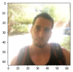
i = random.randint(1,600) # select any random index from 1 to 600
plt.imshow( X_train[i] )
print(y_train[i]) # 0

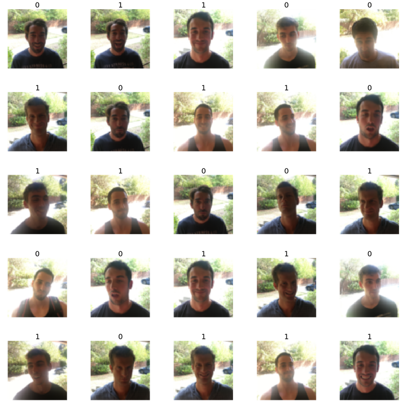
# Let's view more images in a grid format
# Define the dimensions of the plot grid
W_grid = 5
L_grid = 5

# fig, axes = plt.subplots(L_grid, W_grid)
# subplot return the figure object and axes object
# we can use the axes object to plot specific figures at various locations

fig, axes = plt.subplots(L_grid, W_grid, figsize = (25,25))

axes = axes.ravel() # flaten the 15 x 15 matrix into 225 array
# return contiguous(인접한) flattened array(1D array with all the input-array elements and with the same type)

n_training = len(X_train) # get the length of the training dataset

# Select a random number from 0 to n_training
for i in np.arange(0, W_grid * L_grid): # create evenly spaces variables

    # Select a random number
    index = np.random.randint(0, n_training)
    # read and display an image with the selected index    
    axes[i].imshow( X_train[index])
    axes[i].set_title(y_train[index], fontsize = 25)
    #this is showing that 0,1 for reconition of smile or not
    axes[i].axis('off')
    #axis('off') means that remove the coordinate point

plt.subplots_adjust(hspace=0.4)
#subplots_adjust(hspace =0.4) is that adjust distance between pictures

Step 3 MODEL TRAINING

# Let's normalize dataset
X_train = X_train/255
# the picture is indicating from white color
X_test = X_test/255
X_train.shape
#(600, 64, 64, 3)
y_train.shape
# (600,)

# Import train_test_split from scikit library
# tope of tensorflow algorithm
from keras.models import Sequential
# we build neuro network by sequential fashion
from keras.layers import Conv2D, MaxPooling2D, Dense, Flatten, Dropout
# dense for full connected artificial network whichh is right hand side
from keras.optimizers import Adam
#adam optimzation
from keras.callbacks import TensorBoard
#tensorboard. actual train the model.

cnn_model = Sequential()

cnn_model.add(Conv2D(64, 6, 6, input_shape = (64,64,3), activation='relu'))
# this is convolution layer
# 64 kernal, the dimensition at each is 6 x 6
# input shape that basicaally the shape of the actual image that was feeding to our network
# relu output will be sigmoid funciton but if value is '-'(minus) it gonna be 0
cnn_model.add(MaxPooling2D(pool_size = (2, 2)))
# add max pooling layer
cnn_model.add(Dropout(0.2))
# 20percent randomly dropout

cnn_model.add(Conv2D(64, 5, 5, activation='relu'))
#this is another convolution layer
#we dont want to add input_shape, because it doesnt make sense
# here we dont have a input
# because the output coming out from the upper layer is we're going to
# be fed as an input to this layer

cnn_model.add(MaxPooling2D(pool_size = (2, 2)))

cnn_model.add(Flatten())
cnn_model.add(Dense(output_dim = 128, activation = 'relu')) #output network
#this is the hidden layer, one of the layers within our fully connected layer
cnn_model.add(Dense(output_dim = 1, activation = 'sigmoid'))
#last out in the network, our output dimension 1
#dimension 1 is because we only have one output, kind of binary output.
#the output have to be sigmoid. because after copile,
#the tensorflower have to be calculated in binary

cnn_model.compile(loss ='binary_crossentropy', optimizer=Adam(lr=0.001),metrics =['accuracy'])
#'binary_crossentropy' because our output value is the binary
#if our classifying 10 categories, we used binary_categories
#lr <= learning rate.
#we want to train metrices as accurarcy
epochs = 5
#复数,时期 : how may times we're going to be update
#update 5 times.
history = cnn_model.fit(X_train,
                        y_train,
                        batch_size = 30,
                        nb_epoch = epochs,
                        verbose = 1)
# batch_size means that how many imagees would get to be fed
# batch : 자료를 모아 두었다가 일괄해서 처리하는 자료처리의 형태
#verbose is that how many detailes we're going to be sure we actually performaing the trainig

history
Epoch 1/5
600/600 [==============================] - 9s 15ms/step - loss: 0.2444 - acc: 0.9050
Epoch 2/5
600/600 [==============================] - 9s 14ms/step - loss: 0.2150 - acc: 0.9183
Epoch 3/5
600/600 [==============================] - 9s 15ms/step - loss: 0.1829 - acc: 0.9267
Epoch 4/5
600/600 [==============================] - 9s 15ms/step - loss: 0.1931 - acc: 0.9183
Epoch 5/5
600/600 [==============================] - 9s 15ms/step - loss: 0.1662 - acc: 0.9300

Step 4 EVALUATING THE MODEL

evaluation = cnn_model.evaluate(X_test, y_test)
# evaaluating from the data set
evaluation
# [0.3277119962374369, 0.8799999968210857]
print('Test Accuracy : {:.3f}'.format(evaluation[1]))
# loacation in number one. so we have simply event contain two value zero
# numpy array
# Test Accuracy : 0.880
# get the predictions for the test data
predicted_classes = cnn_model.predict_classes(X_test)
predicted_classes.shape
#bunch of 1 or 0
# guess coming out from the guess train data
# (150, 1)
y_test.shape
# (150,)
L = 5
W = 5
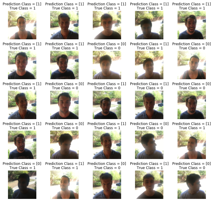
fig, axes = plt.subplots(L, W, figsize = (12,12))
axes = axes.ravel() #

for i in np.arange(0, L * W):  
    axes[i].imshow(X_test[i])
    axes[i].set_title("Prediction Class = {}\n True Class = {}".format(predicted_classes[i], y_test[i]))
    axes[i].axis('off')

plt.subplots_adjust(wspace=0.5)

# axes[i].set_title("Guess{}\n True{}".format(predicted_class[i], y_test[i]))

from sklearn.metrics import confusion_matrix
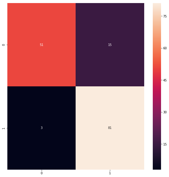
cm = confusion_matrix(y_test, predicted_classes)
plt.figure(figsize = (10,10))
sns.heatmap(cm, annot=True)
# Sum the diagonal element to get the total true correct values

from sklearn.metrics import classification_report

print(classification_report(y_test.T, predicted_classes))

              precision    recall  f1-score   support

           0       0.94      0.77      0.85        66
           1       0.84      0.96      0.90        84

   micro avg       0.88      0.88      0.88       150
   macro avg       0.89      0.87      0.88       150
weighted avg       0.89      0.88      0.88       150


Comment  Read more

15. Polymorphism-Virtual-Functions-Abstracts-Classes

|

Virtual

Exercise

Main.cpp

#include <iostream>
#include "farm.h"

using namespace std;
/* polymorphism, virtual functions, abstract class */
void voiceOfAnimal(Animal *);
void voiceOfAnimal(Animal &);
int main()
{

    Dog dog;
    Cat cat;
    Cow cow;
/*
    cout << animal.getVoice() << endl;
    cout << dog.getVoice() << endl;
    cout << cat.getVoice() << endl;
    cout << cow.getVoice() << endl;
    */
    voiceOfAnimal(&cow); // why we use & because it is for class usually. so it took as reference


    return 0;
}
void voiceOfAnimal(Animal *p)
{
    cout << p->getVoice() << endl;
}
void voiceOfAnimal(Animal &p)
{
    cout << p.getVoice() << endl;
}

farm.h

#ifndef FARM_H_INCLUDED
#define FARM_H_INCLUDED
#include <iostream>

using namespace std;

class Animal
{
        protected:
            string voice;
        public:
            Animal();
            ~Animal();
            virtual string getVoice() = 0; // 가상함수로 선언하여 유도 클래스 Getvoice를 쓸 수 있게 함
};
class Dog : public Animal
{
            string sign;
        public:
            Dog();
            ~Dog();
            string getVoice() { return voice + " " + sign; }
};
class Cat : public Animal
{
            string sign;
        public:
            Cat();
            ~Cat();
            string getVoice() { return voice  + " " +  sign; }
};
class Cow : public Animal
{
            string sign;
        public:
            Cow();
            ~Cow();
            string getVoice() { return voice  + " " +  sign; }
};

#endif // FARM_H_INCLUDED

farm.cpp

#include "farm.h"


Animal::~Animal()
{

}
Dog::Dog()
{
    sign = "D";
    voice = "hau";
}
Dog::~Dog()
{

}
Cat::Cat()
{
    sign = "C";
    voice = "meow";
}
Cat::~Cat()
{

}
Cow::Cow()
{
    sign = "CO";
    voice = "moooo";
}
Cow::~Cow()
{

}

Virtual destructor

  • First of all, it call Dog Class as sub-class within Dynamic
  • then it call Animal Class as Base-Class within pointer. because of it instance called by dynamic

main.cpp

#include <iostream>
#include "farm.h"

using namespace std;
/* virtual destructor */
void voiceOfAnimal(Animal *);
void voiceOfAnimal(Animal &);
int main()
{
/*
    Dog dog;
    Cat cat;
    Cow cow;

    cout << animal.getVoice() << endl;
    cout << dog.getVoice() << endl;
    cout << cat.getVoice() << endl;
    cout << cow.getVoice() << endl;

    voiceOfAnimal(&cow);

*/
    Animal *dog = new Dog;

    delete dog;
    return 0;
}
void voiceOfAnimal(Animal *p)
{
    cout << p->getVoice() << endl;
}
void voiceOfAnimal(Animal &p)
{
    cout << p.getVoice() << endl;
}

farm.h

#ifndef FARM_H_INCLUDED
#define FARM_H_INCLUDED
#include <iostream>

using namespace std;

class Animal
{
        protected:
            string voice;
        public:
            Animal();
            virtual ~Animal();
            virtual string getVoice() = 0;
};
class Dog : public Animal
{
            string sign;
        public:
            Dog();
            ~Dog();
            string getVoice() { return voice + " " + sign; }
};
class Cat : public Animal
{
            string sign;
        public:
            Cat();
            ~Cat();
            string getVoice() { return voice  + " " +  sign; }
};
class Cow : public Animal
{
            string sign;
        public:
            Cow();
            ~Cow();
            string getVoice() { return voice  + " " +  sign; }
};

#endif // FARM_H_INCLUDED

farm.cpp

#include "farm.h"

Animal::Animal()
{

}
Animal::~Animal()
{
    cout << "im from the base class " << endl;
}
Dog::Dog()
{
    sign = "D";
    voice = "hau";
}
Dog::~Dog()
{
    cout << "im from the sub-class " << endl;
}
Cat::Cat()
{
    sign = "C";
    voice = "meow";
}
Cat::~Cat()
{
    cout << "im from the sub-class " << endl;
}
Cow::Cow()
{
    sign = "CO";
    voice = "moooo";
}
Cow::~Cow()
{
    cout << "im from the sub-class " << endl;
}

Comment  Read more

14. Inheritance-between-Classes

|

(Protected)[http://nlp.kookmin.ac.kr/sskang/lect/cpp/ppp.htm]

  • 보호(protected) 멤버
    1. 필요성
    • 파생클래스에게만 접근이 허용되는 비공개(private) 멤버 2. 속성
    • 기본클래스의 비공개(private) 멤버의 속성을 그대로 유지
    • 다만, 파생클래스의 접근이 허용된다는 점만이 private과 다름!

기본클래스 접근 방식 : private, public, protected

  1. 기본클래스를 public으로 접근할 때 : 원래대로 유지
    • 기본클래스의 공개(public) 멤버 –> 파생플래스의 공개(public) 멤버
    • 기본클래스의 보호(protected) 멤버 –> 파생플래스의 보호(protected) 멤버
  2. 기본클래스를 private으로 접근할 때 : 모두 private으로
    • 기본클래스의 공개(public) 멤버 –> 파생플래스의 비공개(private) 멤버
    • 기본클래스의 보호(protected) 멤버 –> 파생플래스의 비공개(private) 멤버
  3. 기본클래스를 protected로 접근할 때 : 모두 protected로
    • 기본클래스의 공개(public) 멤버 –> 파생플래스의 보호(protected) 멤버
    • 기본클래스의 보호(protected) 멤버 –> 파생플래스의 보호(protected) 멤버
    • 어떤 경우든 기본클래스의 private 멤버들은 파생클래스에 의해 접근될 수 없음!

Exercise

Main.cpp

#include <iostream>
#include "point.h"

using namespace std;
/* inheritance between classes */

void operationOnPoints();

int main()
{
    operationOnPoints();

    return 0;
}
void operationOnPoints()
{
    Point2D p2(10, 67);

    p2.Point::setX(5);

    cout << p2.getX() << endl;
    cout << p2.getY() << endl;
}


point.h

#ifndef POINT_H_INCLUDED
#define POINT_H_INCLUDED

class Point //base, parent, superclass
{
    protected:
        int x;
    public:
        Point(int =0);
        ~Point();
        int getX() { return x; }
        void setX(int);
};
class Point2D : public Point //derived, child, subclass
{
    protected:
        int y;
    public:
        Point2D(int =0, int =0);
        ~Point2D();
        int getY() { return y; }
        void setY(int);
        void setX(int);
        void setXY(int, int);

};
class Point3D : public Point2D
{

};

/*
    class Point2D : public Point
    everything what is inside Point (excluding constructor and destructor) will be in Point2D
    private - CANNOT ACCESS
    protected - protected
    public - public

    class Point2D : protected Point
    everything what is inside Point (excluding constructor and destructor) will be in Point2D
    private - CANNOT ACCESS
    protected - protected
    public - protected


    class Point2D : private Point
    everything what is inside Point (excluding constructor and destructor) will be in Point2D
    private - CANNOT ACCESS
    protected - private
    public - private

*/
#endif // POINT_H_INCLUDED

point.cpp

#include <iostream>
#include "point.h"


using namespace std;

Point::Point(int x)
{
    this->x = x;
    cout << "The constructor from the Point class has just been invoked" << endl;
}
Point::~Point()
{
    cout << "The destructor from the Point class has just been invoked" << endl;
}
void Point::setX(int x)
{
    this->x = x;
    cout << "Im from Point" << endl;
}

Point2D::Point2D(int x, int y) : Point(x) // parents
{
    this->y = y;
    cout << "The constructor from the Point2D class has just been invoked" << endl;
}
Point2D::~Point2D()
{
    cout << "The destructor from the Point2D class has just been invoked" << endl;
}

void Point2D::setY(int y)
{
    this->y = y;
}
void Point2D::setXY(int x, int y)
{
    setX(x);
    setY(y);
}
void Point2D::setX(int x)
{
    this->x = x;
    cout << "Im from Point2D" << endl;
}

Comment  Read more

14. BREAST CANCER CLASSIFICATION

|

PROBLEM STATEMENT

  • Predicting if the cancer diagnosis is benign or malignant based on several observations/features
  • 30 features are used, examples:
    • radius (mean of distances from center to points on the perimeter 주의)
    • texture (standard deviation of gray-scale values)
    • perimeter(外缘)
    • area
    • smoothness (local variation in radius lengths)
    • compactness (perimeter^2 / area - 1.0)
    • concavity (severity of concave(凹面的) portions of the contour)
    • concave points (number of concave portions of the contour)
    • symmetry
    • fractal(分形) dimension (“coastline approximation” - 1)
  • Datasets are linearly separable using all 30 input features
  • Number of Instances: 569
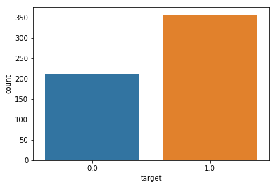
  • Class Distribution: 212 Malignant(恶性的), 357 Benign(善良的;)
  • Target Class
    • Malignant
    • Benign
  • https://archive.ics.uci.edu/ml/datasets/Breast+Cancer+Wisconsin+(Diagnostic)

Step 1 Importing data

# import libraries
import pandas as pd # Import Pandas for data manipulation using dataframes
import numpy as np # Import Numpy for data statistical analysis
import matplotlib.pyplot as plt # Import matplotlib for data visualisation
import seaborn as sns # Statistical data visualization
# %matplotlib inline
# Import Cancer data drom the Sklearn library
from sklearn.datasets import load_breast_cancer
cancer = load_breast_cancer()
cancer
{'data': array([[1.799e+01, 1.038e+01, 1.228e+02, ..., 2.654e-01, 4.601e-01,
         1.189e-01],
        [2.057e+01, 1.777e+01, 1.329e+02, ..., 1.860e-01, 2.750e-01,
         8.902e-02],
        [1.969e+01, 2.125e+01, 1.300e+02, ..., 2.430e-01, 3.613e-01,
         8.758e-02],
        ...,
        [1.660e+01, 2.808e+01, 1.083e+02, ..., 1.418e-01, 2.218e-01,
         7.820e-02],
        [2.060e+01, 2.933e+01, 1.401e+02, ..., 2.650e-01, 4.087e-01,
         1.240e-01],
        [7.760e+00, 2.454e+01, 4.792e+01, ..., 0.000e+00, 2.871e-01,
         7.039e-02]]),
 'target': array([0, 0, 0, 0, 0, 0, 0, 0, 0, 0, 0, 0, 0, 0, 0, 0, 0, 0, 0, 1, 1, 1,
        0, 0, 0, 0, 0, 0, 0, 0, 0, 0, 0, 0, 0, 0, 0, 1, 0, 0, 0, 0, 0, 0,
        0, 0, 1, 0, 1, 1, 1, 1, 1, 0, 0, 1, 0, 0, 1, 1, 1, 1, 0, 1, 0, 0,
        1, 1, 1, 1, 0, 1, 0, 0, 1, 0, 1, 0, 0, 1, 1, 1, 0, 0, 1, 0, 0, 0,
        1, 1, 1, 0, 1, 1, 0, 0, 1, 1, 1, 0, 0, 1, 1, 1, 1, 0, 1, 1, 0, 1,
        1, 1, 1, 1, 1, 1, 1, 0, 0, 0, 1, 0, 0, 1, 1, 1, 0, 0, 1, 0, 1, 0,
        0, 1, 0, 0, 1, 1, 0, 1, 1, 0, 1, 1, 1, 1, 0, 1, 1, 1, 1, 1, 1, 1,
        1, 1, 0, 1, 1, 1, 1, 0, 0, 1, 0, 1, 1, 0, 0, 1, 1, 0, 0, 1, 1, 1,
        1, 0, 1, 1, 0, 0, 0, 1, 0, 1, 0, 1, 1, 1, 0, 1, 1, 0, 0, 1, 0, 0,
        0, 0, 1, 0, 0, 0, 1, 0, 1, 0, 1, 1, 0, 1, 0, 0, 0, 0, 1, 1, 0, 0,
        1, 1, 1, 0, 1, 1, 1, 1, 1, 0, 0, 1, 1, 0, 1, 1, 0, 0, 1, 0, 1, 1,
        1, 1, 0, 1, 1, 1, 1, 1, 0, 1, 0, 0, 0, 0, 0, 0, 0, 0, 0, 0, 0, 0,
        0, 0, 1, 1, 1, 1, 1, 1, 0, 1, 0, 1, 1, 0, 1, 1, 0, 1, 0, 0, 1, 1,
        1, 1, 1, 1, 1, 1, 1, 1, 1, 1, 1, 0, 1, 1, 0, 1, 0, 1, 1, 1, 1, 1,
        1, 1, 1, 1, 1, 1, 1, 1, 1, 0, 1, 1, 1, 0, 1, 0, 1, 1, 1, 1, 0, 0,
        0, 1, 1, 1, 1, 0, 1, 0, 1, 0, 1, 1, 1, 0, 1, 1, 1, 1, 1, 1, 1, 0,
        0, 0, 1, 1, 1, 1, 1, 1, 1, 1, 1, 1, 1, 0, 0, 1, 0, 0, 0, 1, 0, 0,
        1, 1, 1, 1, 1, 0, 1, 1, 1, 1, 1, 0, 1, 1, 1, 0, 1, 1, 0, 0, 1, 1,
        1, 1, 1, 1, 0, 1, 1, 1, 1, 1, 1, 1, 0, 1, 1, 1, 1, 1, 0, 1, 1, 0,
        1, 1, 1, 1, 1, 1, 1, 1, 1, 1, 1, 1, 0, 1, 0, 0, 1, 0, 1, 1, 1, 1,
        1, 0, 1, 1, 0, 1, 0, 1, 1, 0, 1, 0, 1, 1, 1, 1, 1, 1, 1, 1, 0, 0,
        1, 1, 1, 1, 1, 1, 0, 1, 1, 1, 1, 1, 1, 1, 1, 1, 1, 0, 1, 1, 1, 1,
        1, 1, 1, 0, 1, 0, 1, 1, 0, 1, 1, 1, 1, 1, 0, 0, 1, 0, 1, 0, 1, 1,
        1, 1, 1, 0, 1, 1, 0, 1, 0, 1, 0, 0, 1, 1, 1, 0, 1, 1, 1, 1, 1, 1,
        1, 1, 1, 1, 1, 0, 1, 0, 0, 1, 1, 1, 1, 1, 1, 1, 1, 1, 1, 1, 1, 1,
        1, 1, 1, 1, 1, 1, 1, 1, 1, 1, 1, 1, 0, 0, 0, 0, 0, 0, 1]),
cancer.keys()
# dict_keys(['data', 'target', 'target_names', 'DESCR', 'feature_names'])
print(cancer['DESCR'])
Breast Cancer Wisconsin (Diagnostic) Database
=============================================

Notes
-----
Data Set Characteristics:
    :Number of Instances: 569

    :Number of Attributes: 30 numeric, predictive attributes and the class

    :Attribute Information:
        - radius (mean of distances from center to points on the perimeter)
        - texture (standard deviation of gray-scale values)
        - perimeter
        - area
        - smoothness (local variation in radius lengths)
        - compactness (perimeter^2 / area - 1.0)
        - concavity (severity of concave portions of the contour)
        - concave points (number of concave portions of the contour)
        - symmetry
        - fractal dimension ("coastline approximation" - 1)

        The mean, standard error, and "worst" or largest (mean of the three
        largest values) of these features were computed for each image,
        resulting in 30 features.  For instance, field 3 is Mean Radius, field
        13 is Radius SE, field 23 is Worst Radius.

        - class:
                - WDBC-Malignant
                - WDBC-Benign

    :Summary Statistics:

    ===================================== ====== ======
                                           Min    Max
    ===================================== ====== ======
    radius (mean):                        6.981  28.11
    texture (mean):                       9.71   39.28
    perimeter (mean):                     43.79  188.5
    area (mean):                          143.5  2501.0
    smoothness (mean):                    0.053  0.163
    compactness (mean):                   0.019  0.345
    concavity (mean):                     0.0    0.427
    concave points (mean):                0.0    0.201
    symmetry (mean):                      0.106  0.304
    fractal dimension (mean):             0.05   0.097
    radius (standard error):              0.112  2.873
    texture (standard error):             0.36   4.885
    perimeter (standard error):           0.757  21.98
    area (standard error):                6.802  542.2
    smoothness (standard error):          0.002  0.031
    compactness (standard error):         0.002  0.135
    concavity (standard error):           0.0    0.396
    concave points (standard error):      0.0    0.053
    symmetry (standard error):            0.008  0.079
    fractal dimension (standard error):   0.001  0.03
    radius (worst):                       7.93   36.04
    texture (worst):                      12.02  49.54
    perimeter (worst):                    50.41  251.2
    area (worst):                         185.2  4254.0
    smoothness (worst):                   0.071  0.223
    compactness (worst):                  0.027  1.058
    concavity (worst):                    0.0    1.252
    concave points (worst):               0.0    0.291
    symmetry (worst):                     0.156  0.664
    fractal dimension (worst):            0.055  0.208
    ===================================== ====== ======

    :Missing Attribute Values: None

    :Class Distribution: 212 - Malignant, 357 - Benign

    :Creator:  Dr. William H. Wolberg, W. Nick Street, Olvi L. Mangasarian

    :Donor: Nick Street

    :Date: November, 1995

This is a copy of UCI ML Breast Cancer Wisconsin (Diagnostic) datasets.
https://goo.gl/U2Uwz2

Features are computed from a digitized image of a fine needle
aspirate (FNA) of a breast mass.  They describe
characteristics of the cell nuclei present in the image.

Separating plane described above was obtained using
Multisurface Method-Tree (MSM-T) [K. P. Bennett, "Decision Tree
Construction Via Linear Programming." Proceedings of the 4th
Midwest Artificial Intelligence and Cognitive Science Society,
pp. 97-101, 1992], a classification method which uses linear
programming to construct a decision tree.  Relevant features
were selected using an exhaustive search in the space of 1-4
features and 1-3 separating planes.

The actual linear program used to obtain the separating plane
in the 3-dimensional space is that described in:
[K. P. Bennett and O. L. Mangasarian: "Robust Linear
Programming Discrimination of Two Linearly Inseparable Sets",
Optimization Methods and Software 1, 1992, 23-34].

This database is also available through the UW CS ftp server:

ftp ftp.cs.wisc.edu
cd math-prog/cpo-dataset/machine-learn/WDBC/

References
----------
   - W.N. Street, W.H. Wolberg and O.L. Mangasarian. Nuclear feature extraction
     for breast tumor diagnosis. IS&T/SPIE 1993 International Symposium on
     Electronic Imaging: Science and Technology, volume 1905, pages 861-870,
     San Jose, CA, 1993.
   - O.L. Mangasarian, W.N. Street and W.H. Wolberg. Breast cancer diagnosis and
     prognosis via linear programming. Operations Research, 43(4), pages 570-577,
     July-August 1995.
   - W.H. Wolberg, W.N. Street, and O.L. Mangasarian. Machine learning techniques
     to diagnose breast cancer from fine-needle aspirates. Cancer Letters 77 (1994)
     163-171.
print(cancer['target_names'])
# Target name only have two malignant ,benign
# ['malignant' 'benign']
print(cancer['target'])
# 0 , 1 is the who has a cancer or not
print(cancer['target'])

# 0 , 1 is the who has a cancer or not

[0 0 0 0 0 0 0 0 0 0 0 0 0 0 0 0 0 0 0 1 1 1 0 0 0 0 0 0 0 0 0 0 0 0 0 0 0
 1 0 0 0 0 0 0 0 0 1 0 1 1 1 1 1 0 0 1 0 0 1 1 1 1 0 1 0 0 1 1 1 1 0 1 0 0
 1 0 1 0 0 1 1 1 0 0 1 0 0 0 1 1 1 0 1 1 0 0 1 1 1 0 0 1 1 1 1 0 1 1 0 1 1
 1 1 1 1 1 1 0 0 0 1 0 0 1 1 1 0 0 1 0 1 0 0 1 0 0 1 1 0 1 1 0 1 1 1 1 0 1
 1 1 1 1 1 1 1 1 0 1 1 1 1 0 0 1 0 1 1 0 0 1 1 0 0 1 1 1 1 0 1 1 0 0 0 1 0
 1 0 1 1 1 0 1 1 0 0 1 0 0 0 0 1 0 0 0 1 0 1 0 1 1 0 1 0 0 0 0 1 1 0 0 1 1
 1 0 1 1 1 1 1 0 0 1 1 0 1 1 0 0 1 0 1 1 1 1 0 1 1 1 1 1 0 1 0 0 0 0 0 0 0
 0 0 0 0 0 0 0 1 1 1 1 1 1 0 1 0 1 1 0 1 1 0 1 0 0 1 1 1 1 1 1 1 1 1 1 1 1
 1 0 1 1 0 1 0 1 1 1 1 1 1 1 1 1 1 1 1 1 1 0 1 1 1 0 1 0 1 1 1 1 0 0 0 1 1
 1 1 0 1 0 1 0 1 1 1 0 1 1 1 1 1 1 1 0 0 0 1 1 1 1 1 1 1 1 1 1 1 0 0 1 0 0
 0 1 0 0 1 1 1 1 1 0 1 1 1 1 1 0 1 1 1 0 1 1 0 0 1 1 1 1 1 1 0 1 1 1 1 1 1
 1 0 1 1 1 1 1 0 1 1 0 1 1 1 1 1 1 1 1 1 1 1 1 0 1 0 0 1 0 1 1 1 1 1 0 1 1
 0 1 0 1 1 0 1 0 1 1 1 1 1 1 1 1 0 0 1 1 1 1 1 1 0 1 1 1 1 1 1 1 1 1 1 0 1
 1 1 1 1 1 1 0 1 0 1 1 0 1 1 1 1 1 0 0 1 0 1 0 1 1 1 1 1 0 1 1 0 1 0 1 0 0
 1 1 1 0 1 1 1 1 1 1 1 1 1 1 1 0 1 0 0 1 1 1 1 1 1 1 1 1 1 1 1 1 1 1 1 1 1
 1 1 1 1 1 1 1 0 0 0 0 0 0 1]

print(cancer['feature_names'])

['mean radius' 'mean texture' 'mean perimeter' 'mean area'
 'mean smoothness' 'mean compactness' 'mean concavity'
 'mean concave points' 'mean symmetry' 'mean fractal dimension'
 'radius error' 'texture error' 'perimeter error' 'area error'
 'smoothness error' 'compactness error' 'concavity error'
 'concave points error' 'symmetry error' 'fractal dimension error'
 'worst radius' 'worst texture' 'worst perimeter' 'worst area'
 'worst smoothness' 'worst compactness' 'worst concavity'
 'worst concave points' 'worst symmetry' 'worst fractal dimension']

print(cancer['data'])
[[1.799e+01 1.038e+01 1.228e+02 ... 2.654e-01 4.601e-01 1.189e-01]
 [2.057e+01 1.777e+01 1.329e+02 ... 1.860e-01 2.750e-01 8.902e-02]
 [1.969e+01 2.125e+01 1.300e+02 ... 2.430e-01 3.613e-01 8.758e-02]
 ...
 [1.660e+01 2.808e+01 1.083e+02 ... 1.418e-01 2.218e-01 7.820e-02]
 [2.060e+01 2.933e+01 1.401e+02 ... 2.650e-01 4.087e-01 1.240e-01]
 [7.760e+00 2.454e+01 4.792e+01 ... 0.000e+00 2.871e-01 7.039e-02]]
cancer['data'].shape #(569, 30)
#569 raw as data set, 30 is the 30 feature.
df_cancer = pd.DataFrame(np.c_[cancer['data'], cancer['target']], columns = np.append(cancer['feature_names'], ['target']))
# append two vecotr or two columns together. so we can have cancer name and target as well
# to make better dataframe, we use that.
# which means 30 columns all the data we had
# then can additional column withch the first column that includes a target data wich is kind of you know we can include all the trains the in put and output
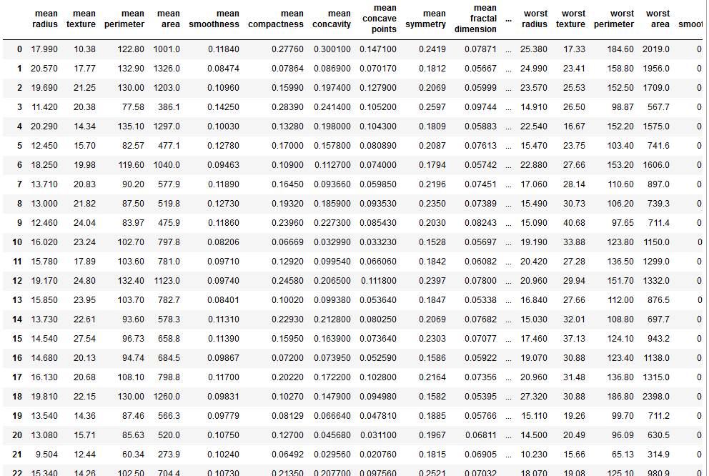
df_cancer.head()
#it showing our goal 'target'

x = np.array([1,2,3])
x.shape
# (3,)
Example = np.c_[np.array([1,2,3]), np.array([4,5,6])]
Example.shape
# (3, 2)

Step 2 Visualize data

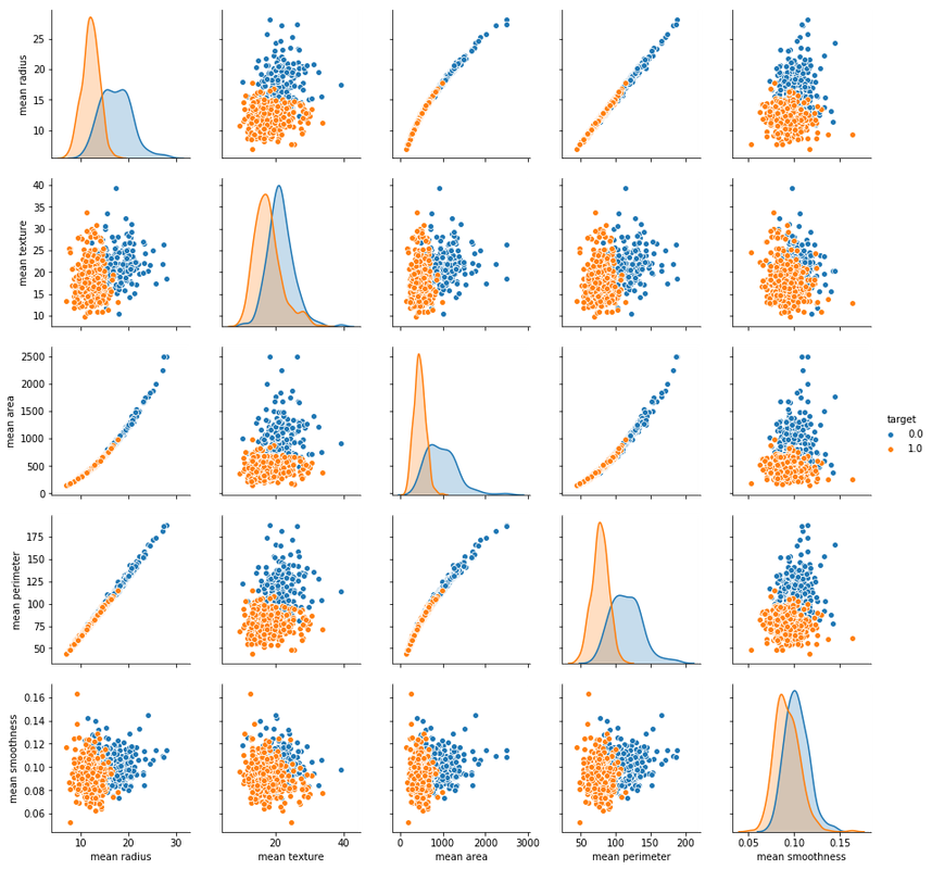
sns.pairplot(df_cancer, hue = 'target', vars = ['mean radius', 'mean texture', 'mean area', 'mean perimeter', 'mean smoothness'] )
# hue is the target of the data what we want to know about it

sns.countplot(df_cancer['target'], label = "Count")

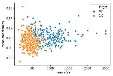
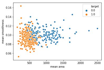
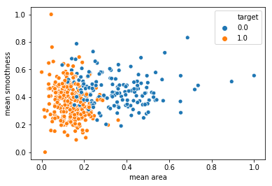
sns.scatterplot(x = 'mean area', y = 'mean smoothness', hue = 'target', data = df_cancer)

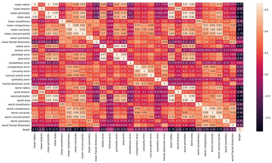
# Let's check the correlation between the variables
# Strong correlation between the mean radius and mean perimeter, mean area and mean primeter
plt.figure(figsize=(20,10))
sns.heatmap(df_cancer.corr(), annot=True)

Step 3 MODEL TRAINING (FINDING A PROBLEM SOLUTION)


# Let's drop the target label coloumns because we only need input data.
# target data is output we created
# axis=1 is we all delete data of target
X = df_cancer.drop(['target'],axis=1)
X

y = df_cancer['target']
y
0      0.0
1      0.0
2      0.0
3      0.0
4      0.0
5      0.0
6      0.0
7      0.0
8      0.0
9      0.0
10     0.0
11     0.0
12     0.0
13     0.0
14     0.0
15     0.0
16     0.0
17     0.0
18     0.0
19     1.0
20     1.0
21     1.0
22     0.0
23     0.0
24     0.0
25     0.0
26     0.0
27     0.0
28     0.0
29     0.0
      ...
from sklearn.model_selection import train_test_split

X_train, X_test, y_train, y_test = train_test_split(X, y, test_size = 0.20, random_state=5)

# random_state is the just seed
X_train.shape # (455, 30)
X_test.shape # (114, 30)
y_train.shape # (455,)
y_test.shape # (114,)

from sklearn.svm import SVC #support vector machine learning
from sklearn.metrics import classification_report, confusion_matrix
#confusion_matrix 오차 행렬
#matrix inside for moving foward

svc_model = SVC()
svc_model.fit(X_train, y_train)
from sklearn.svm import SVC #support vector machine learning

from sklearn.metrics import classification_report, confusion_matrix

#confusion_matrix 오차 행렬

#matrix inside for moving foward

​

svc_model = SVC()

svc_model.fit(X_train, y_train)

SVC(C=1.0, cache_size=200, class_weight=None, coef0=0.0,
  decision_function_shape='ovr', degree=3, gamma='auto', kernel='rbf',
  max_iter=-1, probability=False, random_state=None, shrinking=True,
  tol=0.001, verbose=False)

Step 4 EVALUATING THE MODEL

y_predict = svc_model.predict(X_test)
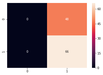
cm = confusion_matrix(y_test, y_predict)
sns.heatmap(cm, annot=True)
#annot is the showing the value
#showing that there is the a lot of the error

print(classification_report(y_test, y_predict))
precision    recall  f1-score   support

0.0       0.00      0.00      0.00        48
1.0       0.58      1.00      0.73        66

avg / total       0.34      0.58      0.42       114

Step 5 Improving the model

min_train = X_train.min()
#we are going to normalize the x-train. just get minimum value
min_train
mean radius                  6.981000
mean texture                 9.710000
mean perimeter              43.790000
mean area                  143.500000
mean smoothness              0.052630
mean compactness             0.019380
mean concavity               0.000000
mean concave points          0.000000
mean symmetry                0.106000
mean fractal dimension       0.049960
radius error                 0.111500
texture error                0.362100
perimeter error              0.757000
area error                   6.802000
smoothness error             0.001713
compactness error            0.002252
concavity error              0.000000
concave points error         0.000000
symmetry error               0.007882
fractal dimension error      0.000950
worst radius                 7.930000
worst texture               12.020000
worst perimeter             50.410000
worst area                 185.200000
worst smoothness             0.071170
worst compactness            0.027290
worst concavity              0.000000
worst concave points         0.000000
worst symmetry               0.156500
worst fractal dimension      0.055040
dtype: float64
range_train = (X_train - min_train).max()
#range to get maximum value of range_train
range_train
mean radius                  21.129000
mean texture                 29.570000
mean perimeter              144.710000
mean area                  2355.500000
mean smoothness               0.110770
mean compactness              0.326020
mean concavity                0.426800
mean concave points           0.201200
mean symmetry                 0.198000
mean fractal dimension        0.045790
radius error                  2.761500
texture error                 4.522900
perimeter error              21.223000
area error                  518.798000
smoothness error              0.029417
compactness error             0.133148
concavity error               0.396000
concave points error          0.052790
symmetry error                0.071068
fractal dimension error       0.028890
worst radius                 25.190000
worst texture                37.520000
worst perimeter             170.390000
worst area                 3246.800000
worst smoothness              0.129430
worst compactness             1.030710
worst concavity               1.105000
worst concave points          0.291000
worst symmetry                0.420900
worst fractal dimension       0.152460
dtype: float64
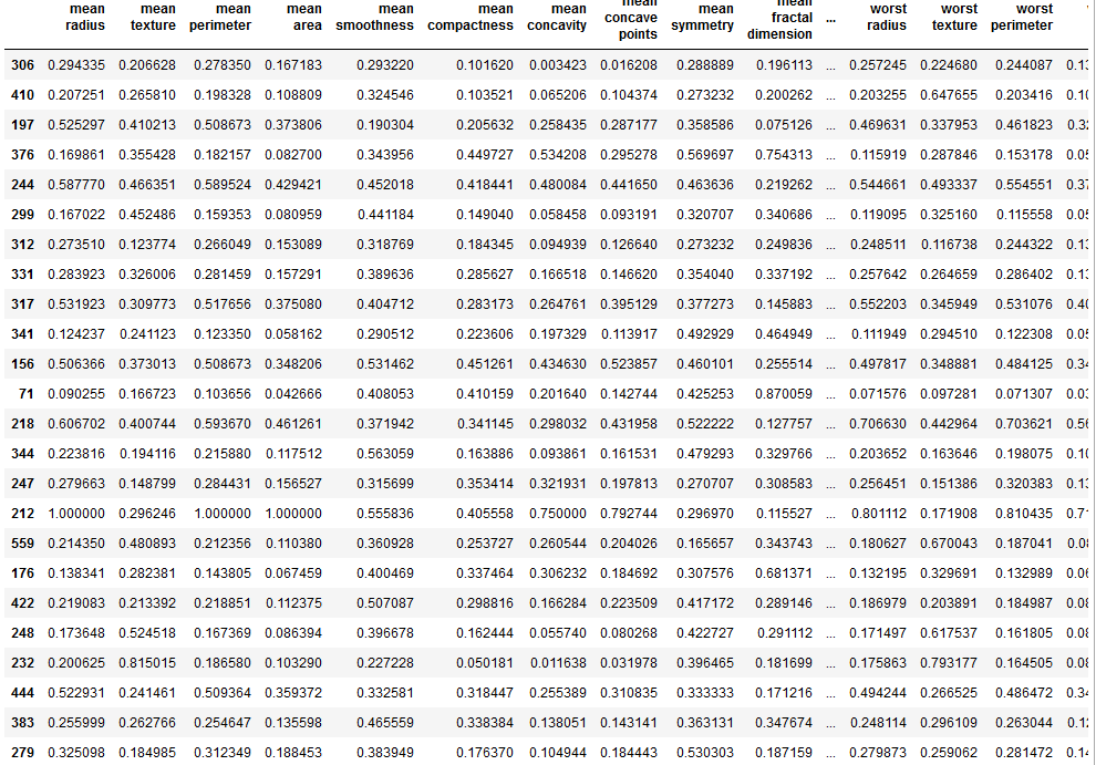
X_train_scaled = (X_train - min_train)/range_train
X_train_scaled

sns.scatterplot(x = X_train['mean area'], y = X_train['mean smoothness'], hue = y_train)

sns.scatterplot(x = X_train_scaled['mean area'], y = X_train_scaled['mean smoothness'], hue = y_train)

min_test = X_test.min()
range_test = (X_test - min_test).max()
X_test_scaled = (X_test - min_test)/range_test
from sklearn.svm import SVC
from sklearn.metrics import classification_report, confusion_matrix

svc_model = SVC()
svc_model.fit(X_train_scaled, y_train)

y_predict = svc_model.predict(X_test_scaled) # we use new data set. because the
# before normailzation, data is not good.
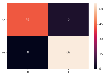
cm = confusion_matrix(y_test, y_predict)

sns.heatmap(cm,annot=True,fmt="d")
#fmt

print(classification_report(y_test,y_predict))
#to make classification_report.
#recall is how much well catch the true or not
#precision is how much good predict
         precision    recall  f1-score   support

0.0       1.00      0.90      0.95        48
1.0       0.93      1.00      0.96        66

avg / total       0.96      0.96      0.96       114


Step 5 Improving the model part 2

param_grid = {'C': [0.1, 1, 10, 100], 'gamma': [1, 0.1, 0.01, 0.001], 'kernel': ['rbf']}


#define our range.
# learning rate C and Gamma of blanket
#'C' parameter
# kernal is the basic function.

from sklearn.model_selection import GridSearchCV
#optimization for model

grid = GridSearchCV(SVC(),param_grid,refit=True,verbose=4)
# how many value we want to display that verbos , 4 ,5 what ever for our grid
# refit an estimator(추정법칙) using the best found parameters on the whole dataset
# verbose(冗长的)

grid.fit(X_train_scaled,y_train)
#seaching for best value of gamma and c
Fitting 3 folds for each of 16 candidates, totalling 48 fits
[CV] C=0.1, gamma=1, kernel=rbf ......................................
[CV]  C=0.1, gamma=1, kernel=rbf, score=0.9671052631578947, total=   0.0s
[CV] C=0.1, gamma=1, kernel=rbf ......................................
[CV]  C=0.1, gamma=1, kernel=rbf, score=0.9210526315789473, total=   0.0s
[CV] C=0.1, gamma=1, kernel=rbf ......................................
[CV]  C=0.1, gamma=1, kernel=rbf, score=0.9470198675496688, total=   0.0s
[CV] C=0.1, gamma=0.1, kernel=rbf ....................................
[CV]  C=0.1, gamma=0.1, kernel=rbf, score=0.9144736842105263, total=   0.0s
[CV] C=0.1, gamma=0.1, kernel=rbf ....................................
[CV]  C=0.1, gamma=0.1, kernel=rbf, score=0.8881578947368421, total=   0.0s
[CV] C=0.1, gamma=0.1, kernel=rbf ....................................
[CV]  C=0.1, gamma=0.1, kernel=rbf, score=0.8675496688741722, total=   0.0s
[CV] C=0.1, gamma=0.01, kernel=rbf ...................................
[CV]  C=0.1, gamma=0.01, kernel=rbf, score=0.6381578947368421, total=   0.0s
[CV] C=0.1, gamma=0.01, kernel=rbf ...................................
[CV]  C=0.1, gamma=0.01, kernel=rbf, score=0.6381578947368421, total=   0.0s
[CV] C=0.1, gamma=0.01, kernel=rbf ...................................
[CV]  C=0.1, gamma=0.01, kernel=rbf, score=0.6423841059602649, total=   0.0s
[CV] C=0.1, gamma=0.001, kernel=rbf ..................................
[CV]  C=0.1, gamma=0.001, kernel=rbf, score=0.6381578947368421, total=   0.0s
[CV] C=0.1, gamma=0.001, kernel=rbf ..................................
[CV]  C=0.1, gamma=0.001, kernel=rbf, score=0.6381578947368421, total=   0.0s
[CV] C=0.1, gamma=0.001, kernel=rbf ..................................
[CV]  C=0.1, gamma=0.001, kernel=rbf, score=0.6423841059602649, total=   0.0s
[CV] C=1, gamma=1, kernel=rbf ........................................
[CV]  C=1, gamma=1, kernel=rbf, score=0.993421052631579, total=   0.0s
[CV] C=1, gamma=1, kernel=rbf ........................................
[CV]  C=1, gamma=1, kernel=rbf, score=0.9473684210526315, total=   0.0s
[CV] C=1, gamma=1, kernel=rbf ........................................
[CV]  C=1, gamma=1, kernel=rbf, score=0.9801324503311258, total=   0.0s
[CV] C=1, gamma=0.1, kernel=rbf ......................................
[CV]  C=1, gamma=0.1, kernel=rbf, score=0.9736842105263158, total=   0.0s
[CV] C=1, gamma=0.1, kernel=rbf ......................................
[CV]  C=1, gamma=0.1, kernel=rbf, score=0.9276315789473685, total=   0.0s
[CV] C=1, gamma=0.1, kernel=rbf ......................................
[CV]  C=1, gamma=0.1, kernel=rbf, score=0.9403973509933775, total=   0.0s
[CV] C=1, gamma=0.01, kernel=rbf .....................................
[CV]  C=1, gamma=0.01, kernel=rbf, score=0.9144736842105263, total=   0.0s
grid.best_params_
# {'C': 10, 'gamma': 0.1, 'kernel': 'rbf'}
grid.best_estimator_
SVC(C=10, cache_size=200, class_weight=None, coef0=0.0,
  decision_function_shape='ovr', degree=3, gamma=0.1, kernel='rbf',
  max_iter=-1, probability=False, random_state=None, shrinking=True,
  tol=0.001, verbose=False)
grid_predictions = grid.predict(X_test_scaled)
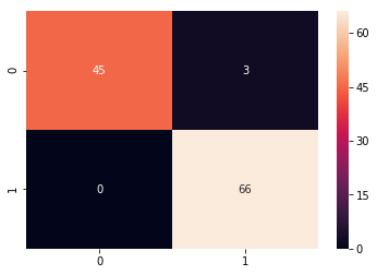
cm = confusion_matrix(y_test, grid_predictions)
sns.heatmap(cm, annot=True)

print(classification_report(y_test,grid_predictions))
precision    recall  f1-score   support

0.0       1.00      0.94      0.97        48
1.0       0.96      1.00      0.98        66

avg / total       0.97      0.97      0.97       114


Comment  Read more

13. Predicting Revenue Using Simple Linear Regression

|

PROBLEM STATEMENT

  • You own an ice cream business and you would like to create a model that could predict the daily revenue in dollars based on the outside air temperature (degC). You decide that a Linear Regression model might be a good candidate to solve this problem.
  • Data set:
    • Independent variable X: Outside Air Temperature
    • Dependant variable Y: Overall daily revenue generated in dollars

Step 1 Libraries Import

import pandas as pd
import numpy as np
import matplotlib.pyplot as plt
import seaborn as sns
%matplotlib inline
#matplotlib inline, if we execute plot code in notebboot, we can see picture immediatly

Step 2 IMPORT DATASET

IceCream = pd.read_csv("IceCreamData.csv")
IceCream.head(100)
Temperature 	Revenue
0 	24.566884 	534.799028
1 	26.005191 	625.190122
2 	27.790554 	660.632289
3 	20.595335 	487.706960
4 	11.503498 	316.240194
5 	14.352514 	367.940744
6 	13.707780 	308.894518
7 	30.833985 	696.716640
8 	0.976870 	55.390338
9 	31.669465 	737.800824
10 	11.455253 	325.968408
11 	3.664670 	71.160153
12 	18.811824 	467.446707
13 	13.624509 	289.540934
14 	39.539909 	905.477604
15 	18.483141 	469.909033
16 	25.935375 	648.209998
IceCream.tail()
Temperature 	Revenue
495 	22.274899 	524.746364
496 	32.893092 	755.818399
497 	12.588157 	306.090719
498 	22.362402 	566.217304
499 	28.957736 	655.660388
IceCream.describe()
Temperature 	Revenue
count 	500.000000 	500.000000
mean 	22.232225 	521.570777
std 	8.096388 	175.404751
min 	0.000000 	10.000000
25% 	17.122258 	405.558681
50% 	22.392791 	529.368565
75% 	27.740674 	642.257922
max 	45.000000 	1000.000000
IceCream.info()
IceCream.info()

<class 'pandas.core.frame.DataFrame'>
RangeIndex: 500 entries, 0 to 499
Data columns (total 2 columns):
Temperature    500 non-null float64
Revenue        500 non-null float64
dtypes: float64(2)
memory usage: 7.9 KB

Step 3 Visualize Dataset

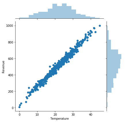
sns.jointplot(x='Temperature', y='Revenue', data = IceCream)
# name have to be exactly same as in data dataframe

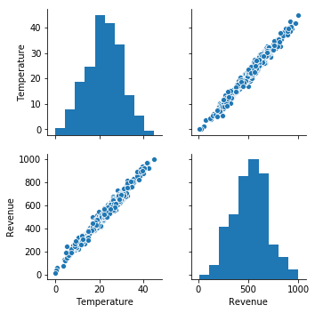
sns.pairplot(IceCream)
#dafaflow nor need here to put X and Y

sns.lmplot(x='Temperature', y='Revenue', data=IceCream)
# plotting linear line wiht line

Step 4 Create Testing And Training Dataset

y = IceCream['Revenue']
X = IceCream['Temperature']
from sklearn.model_selection import train_test_split
X_train, X_test, y_train, y_test = train_test_split(X, y, test_size=0.25)
#define our ratio
#75percent is the train set

Step 5 TRAIN THE MODEL

X_train.shape #(375,)
from sklearn.linear_model import LinearRegression
regressor = LinearRegression(fit_intercept =True)
# we imported the class, 'intercept' meansthat we instantiate with an object
# 'fit_intercept'means we are asking the model to simply update for us not just the slope m but obtain our intercept
# if false, only line only return m value , default will be zero
# intercept 일차함수의 그래프가 축과 만나는 교점의 좌표
regressor.fit(X_train.values.reshape(-1,1),y_train)
#fit the valuable into regression class
print('Linear Model Coefficient (m): ', regressor.coef_) #Linear Model Coefficient (m):  [21.4418582]
print('Linear Model Coefficient (b): ', regressor.intercept_) # Linear Model Coefficient (b):  46.867275700132154
# our y intercept is intercepting the at 47

Step 6 Test The model

y_predict = regressor.predict(X_test.values.reshape(-1,1))
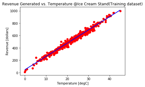
plt.scatter(X_train.values.reshape(-1,1), y_train, color = 'red')
plt.plot(X_train.values.reshape(-1,1), regressor.predict(X_train.values.reshape(-1,1)), color = 'blue')
plt.ylabel('Revenue [dollars]')
plt.xlabel('Temperature [degC]')
plt.title('Revenue Generated vs. Temperature @Ice Cream Stand(Training dataset)')

# VISUALIZE TEST SET RESULTS
plt.scatter(X_test.values.reshape(-1,1), y_test, color = 'red')
plt.plot(X_test.values.reshape(-1,1), regressor.predict(X_test.values.reshape(-1,1)), color = 'blue')
plt.ylabel('Revenue [dollars]')
plt.xlabel('Hours')
plt.title('Revenue Generated vs. Hours @Ice Cream Stand(Test dataset)')

new_x = 30
new_x = np.array(new_x).reshape(1,-1)
y_predict = regressor.predict(new_x)
# 왜냐하면 이미 템프레쳐 트레이닝 데이터가 75퍼로 공부를 시켰기 떄문에
# 30일때 값이 얼마인지 알 수 있다.
y_predict # array([690.1230218])

Sample_T = 35 # this is guessing if temperature 35 in predicting.
Sample_T = np.array(Sample_T).reshape(1,-1)
y_predict = regressor.predict(Sample_T)
y_predict

Comment  Read more