7. One Dimensional Search Methods
07 Oct 2019 | Optimization method
1. GOLDEN SECTION SEARCH
- The search methods we discuss in this and the next section allow us to determine the minimizer of a function f : R —> R over a closed interval, say [$a_o$, $b_o$]
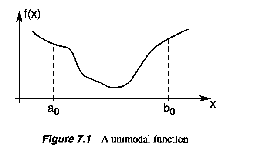
- The only property that we assume of the objective function f is that it is unimodal(단 한가지의 모델)
- which means that f has only one local minimizer
- The methods we discuss are based on evaluating the objective function at different points in the interval [$a_o$, $b_o$]
- We choose these points in such a way that an approximation to the minimizer of / may be achieved in as few evaluations as possible.
- Our goal is to progressively narrow the range until the minimizer is “boxed in” with sufficient accuracy.
- Consider a unimodal function / of one variable and the interval [$a_o$, $b_o$].
- If we evaluate / at only one intermediate point of the interval, we cannot narrow the range within which we know the minimizer is located.
- We have to evaluate f at two intermediate points
- We choose the intermediate points in such a way that the reduction in the range is symmetric, in the sense that:
- We then evaluate f at the intermediate points
-
If f($a_1$) < f($a_2$), then the minimizer
must lie in the range [$a_0$, $b_1$]. If, on the other hand,f($a_1$) >= f($a_2$), then the minimizer
is located in the range [$a_1$, $b_0$]
- Starting with the reduced range of uncertainty we can repeat the process and similarly find two new points, say $a_2$ and $b_2$ using the same value of p < 1/2
- However, we would like to minimize the number of the objective function evaluations while reducing the width of the uncertainty interval.
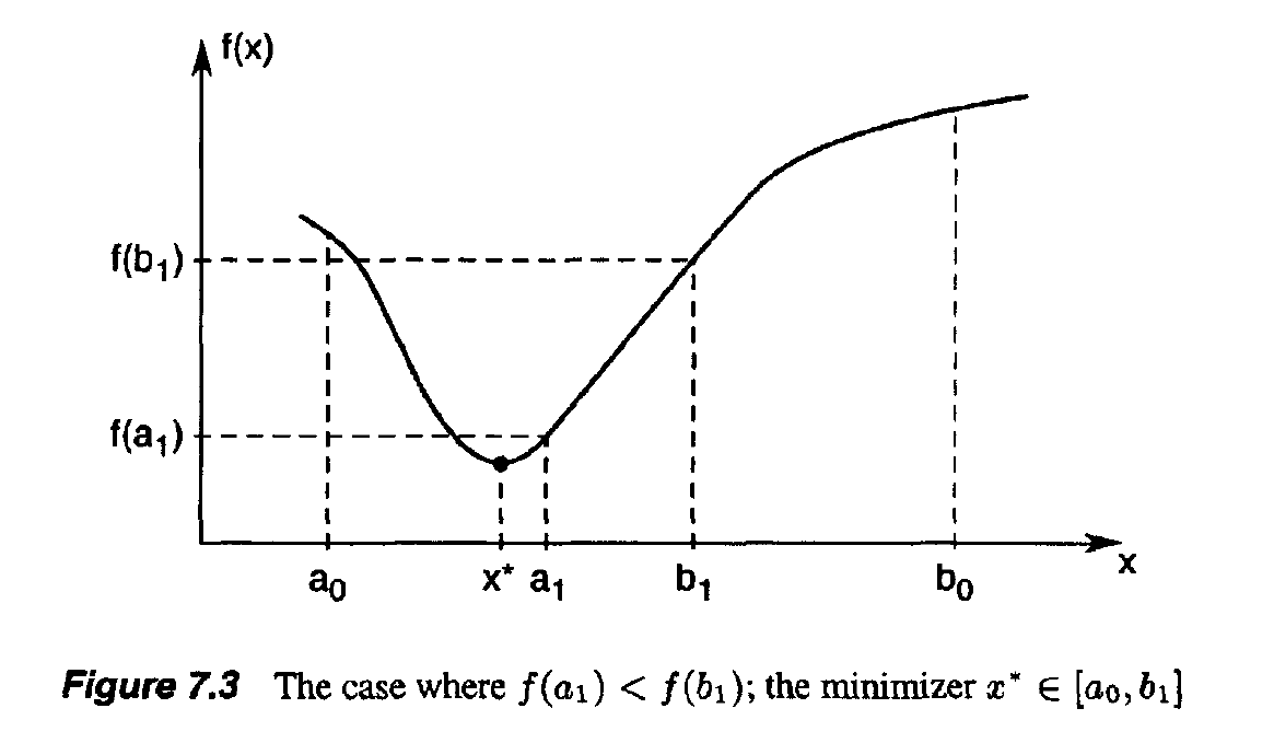
- Suppose, for example, that f($a_1$) < f($b_1$), as in Figure 7.3.
- Because $a_1$ is already in the uncertainty interval and f ( $a_1$ ) is already known, we can make $a_1$
coincide with $b_2$
- Thus, only one new evaluation of f at $a_2$ would be necessary
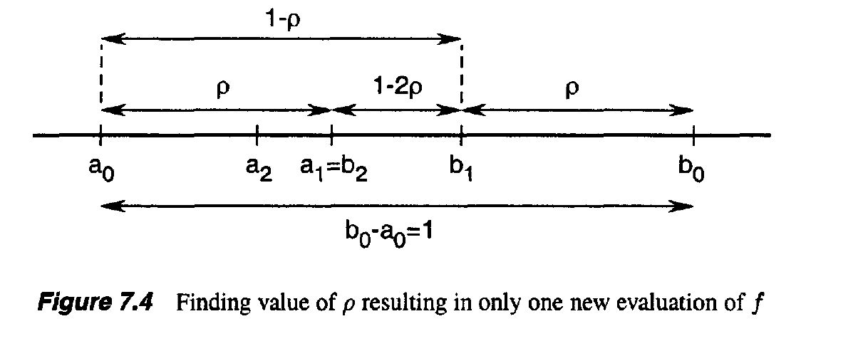
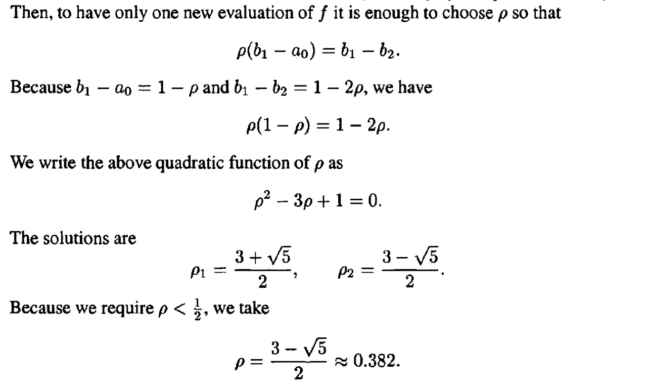
- To find the value of p that results in only one new evaluation of f
- Without loss of generality, imagine that the original range [$a_0$, $b_0$] is of unit length.
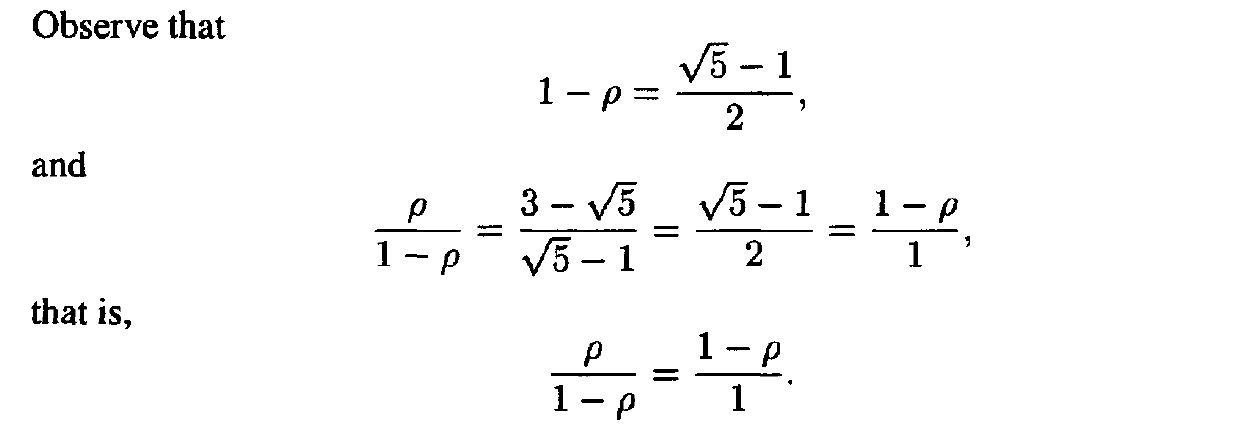
- Thus, dividing a range in the ratio of p to 1 — p has the effect that the ratio of the shorter segment to the longer equals the ratio of the longer to the sum of the two.
- This rule was referred to by ancient Greek geometers as the Golden Section.
- Using this Golden Section rule means that at every stage of the uncertainty range reduction (except the first one), the objective function f need only be evaluated at one new point.
- The uncertainty range is reduced by the ratio 1 — p = 0.61803 at every stage.
- Hence, N steps of reduction using the Golden Section method reduces the range by the factor
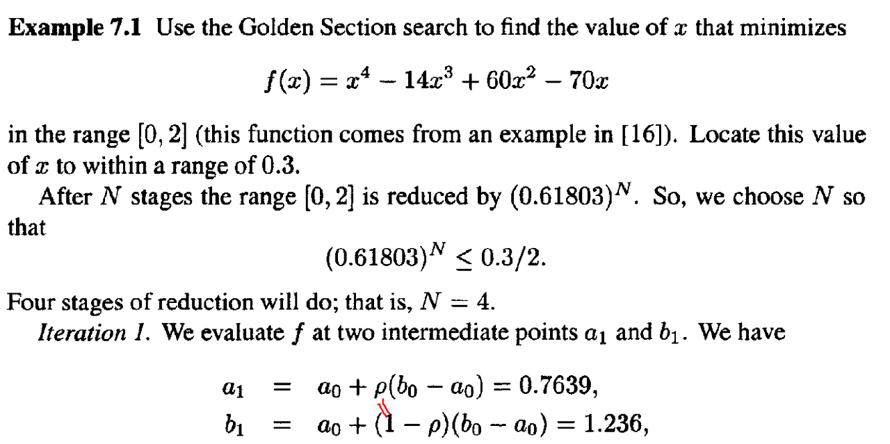
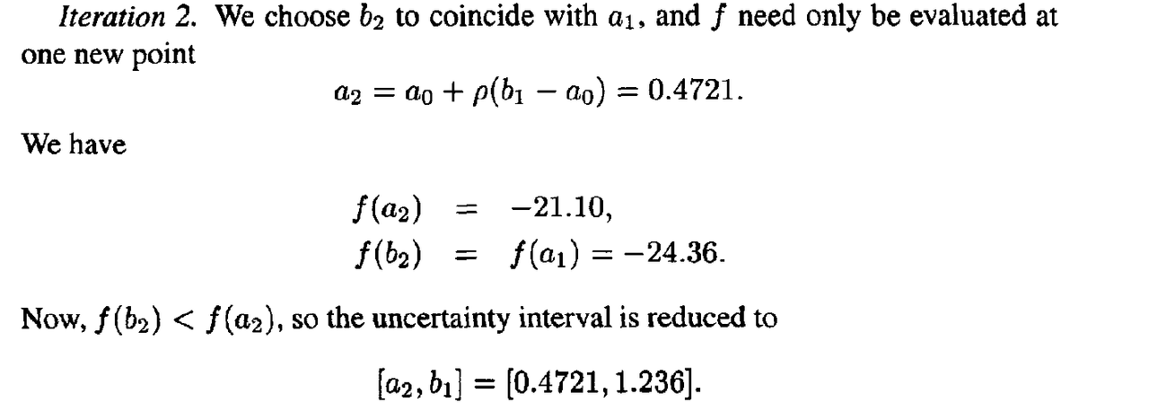
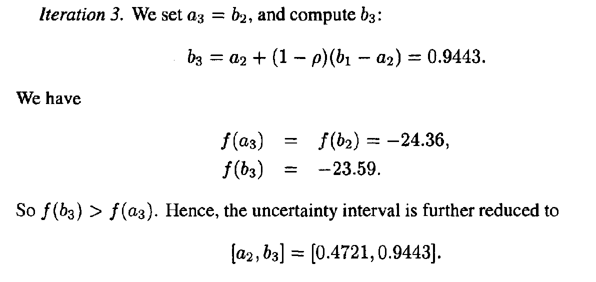
Example
2. FIBONACCI SEARCH
- Recall that the Golden Section method uses the same value of p throughout
- Suppose now that we are allowed to vary the value p from stage to stage, so that at the k th stage in the reduction process we use a value $p_k$, at the next stage we use a value p(k+1), and so on.
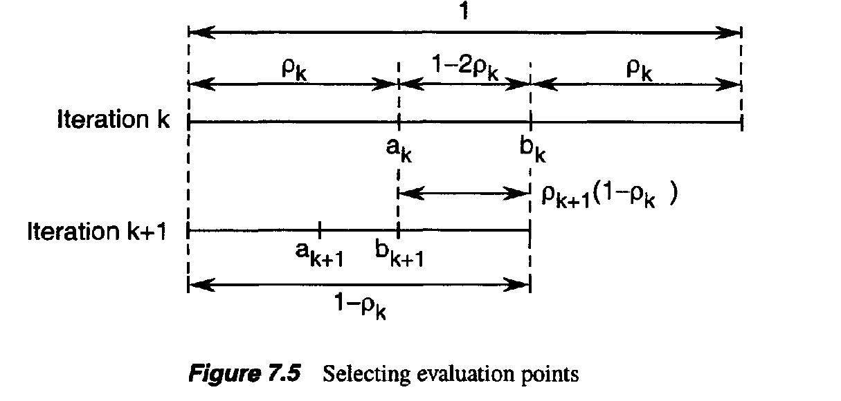
- As in the Golden Section search, our goal is to select successive values of $p_k$, 0 < $P_k$ < 1/2, such that only one new function evaluation is required at each stage.
- From Figure 7.5, we see that it is sufficient to choose the $p_k$ such that:
- There are many sequences $p_1$,$p_2$, • • • that satisfy the above law of formation, and the condition that 0 < $p_k$ < 1/2.
- Suppose that we are given a sequence $p_1$,$p_2$, - - • satisfying the above conditions, and we use this sequence in our search algorithm.
- Then, after N iterations of the algorithm, the uncertainty range is reduced by a factor of
- Depending on the sequence $p_1$,$p_2$,…, we get a different reduction factor.
- The natural question is as follows: What sequence $p_1$,$p_2$,… minimizes the above reduction factor?
- This problem is a constrained optimization problem that can be formally stated:
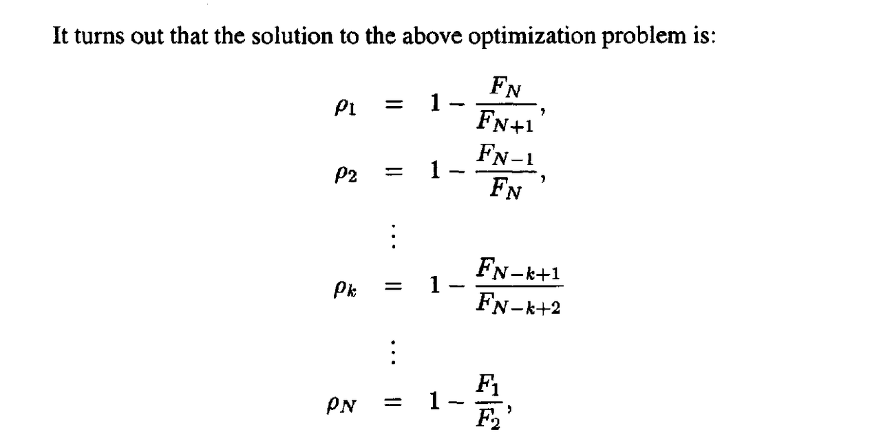
- Before we give the solution to the above optimization problem, we first need to introduce the Fibonacci sequence, FI,F2,F3, — This sequence is defined as follows. First, let F(-1) = 0 and F(0) = 1 by convention. Then, for k > 0,
- where the $F_k$ are the elements of the Fibonacci sequence.
- The resulting algorithm is called the Fibonacci search method.
- In the Fibonacci search method, the uncertainty range is reduced by the factor:
- Because the Fibonacci method uses the optimal values of $p_1$,$p_2$, • • •» the above reduction factor is less than that of the Golden Section method.
- In other words, the Fibonacci method is better than the Golden Section method in that it gives a smaller final uncertainty range.
- We point out that there is an anomaly in the final iteration of the Fibonacci search method, because:
- Recall that we need two intermediate points at each stage, one that comes from a previous iteration and another that is a new evaluation point.
- However, with $p_N$ = 1/2, the two intermediate points coincide in the middle of the uncertainty interval, and therefore we cannot further reduce the uncertainty range.
- To get around, this problem, we perform the new evaluation for the last iteration using $p_N$ = 1/2 - ε, where ε is the small number
- In other words, the new evaluation point is just to the left or right of the midpoint of the uncertainty interval.
- This modification to the Fibonacci method is, of course, of no significant practical consequence
- As a result of the above modification, the reduction in the uncertainty range at the last iteration may be either
- depending on which of the two points has the smaller objective function value.
- Therefore, in the worst case, the reduction factor in the uncertainty range for the Fibonacci method is
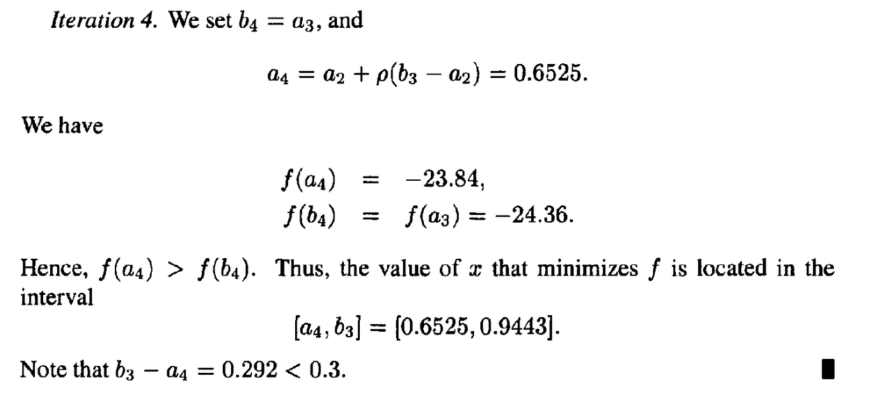
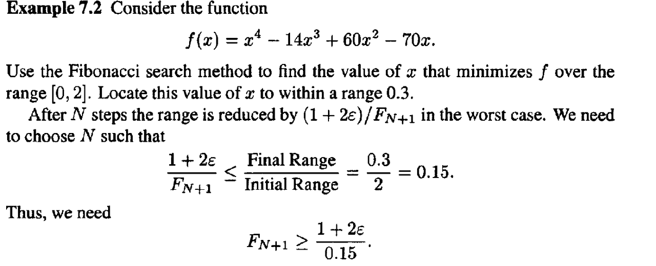
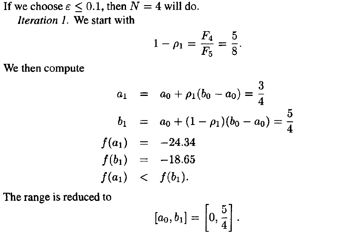
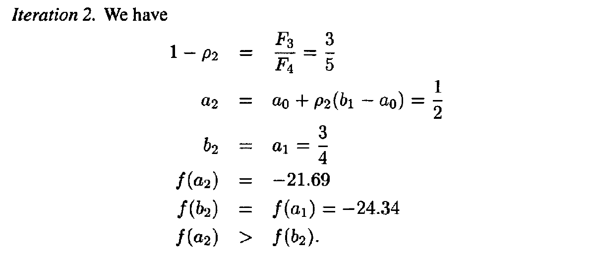
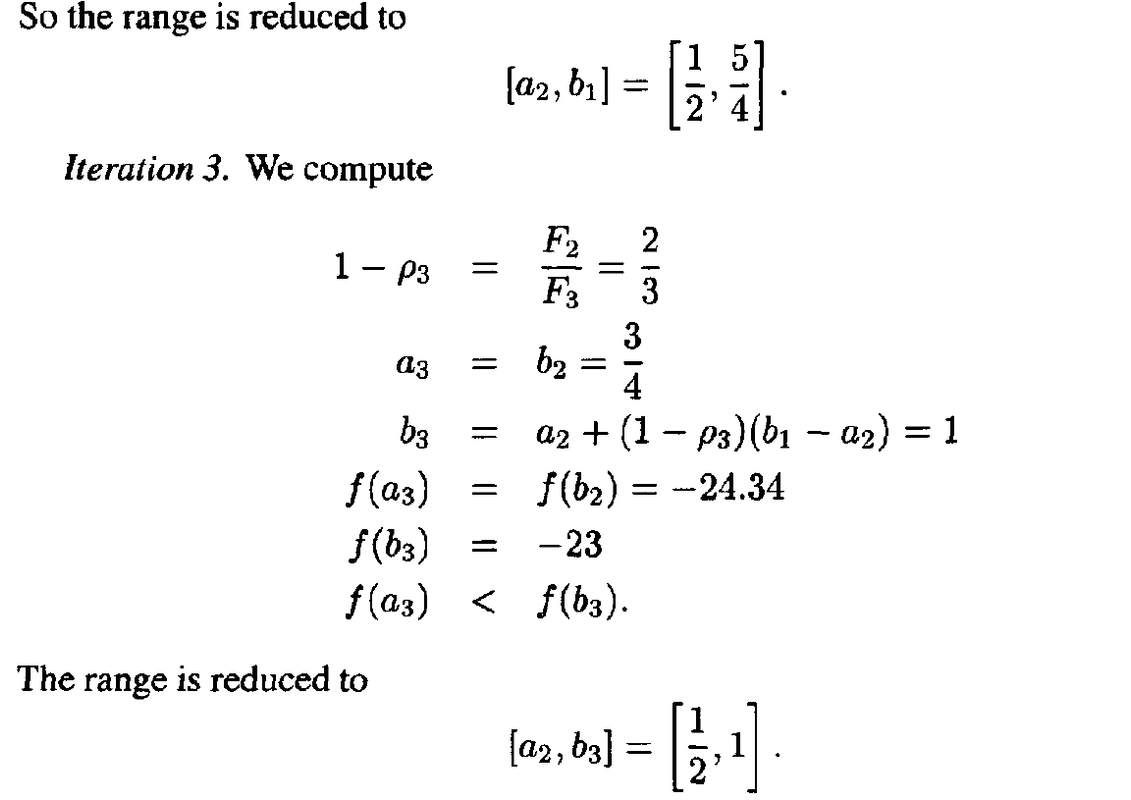
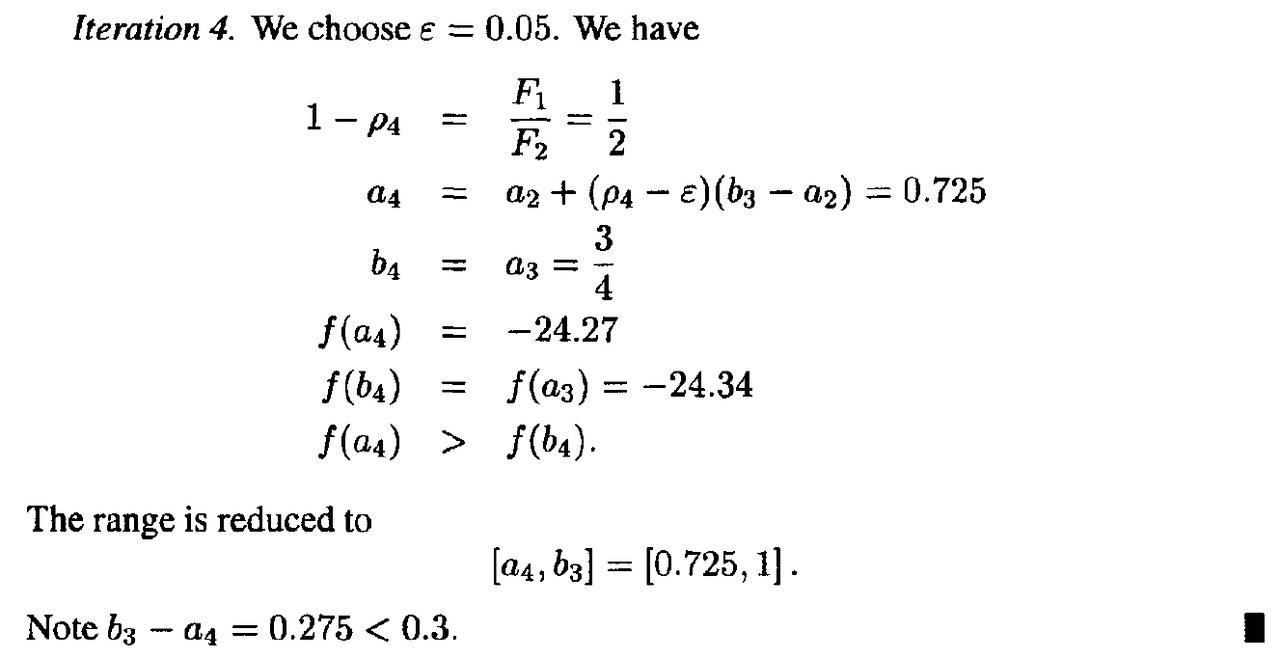
Example
3. NEWTON’S METHOD
- Suppose again that we are confronted(降临于) with the problem of minimizing a function f of a single real variable x.
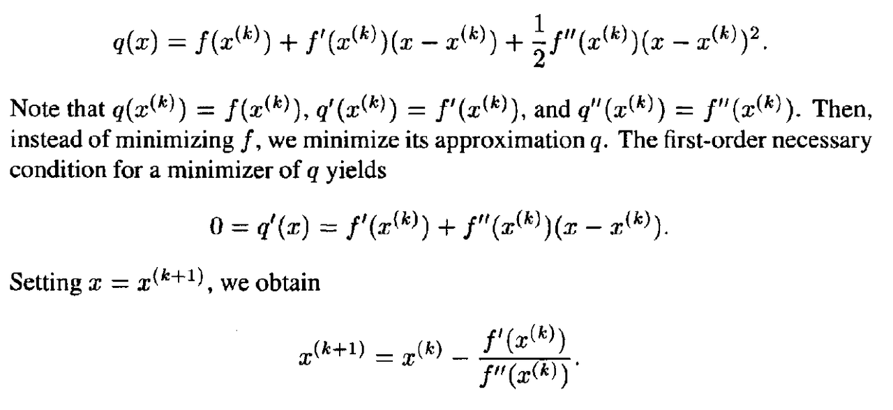
- We assume now that at each measurement point $x^k$ we can calculate f($x^k$), f’’($x^k$}, and f’’’($x^k$). We can fit a quadratic function through $x^k$ that matches its first and second derivatives with that of the function f.
- This quadratic has the form :
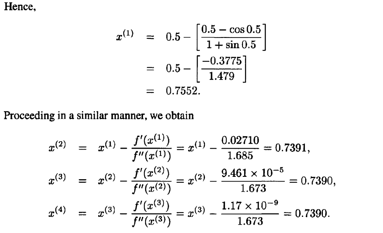
Example 1
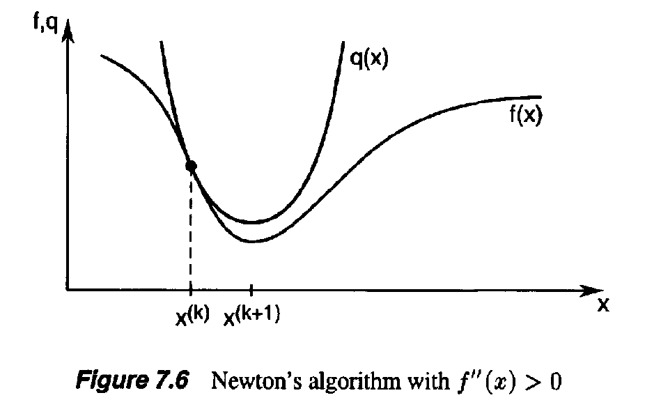
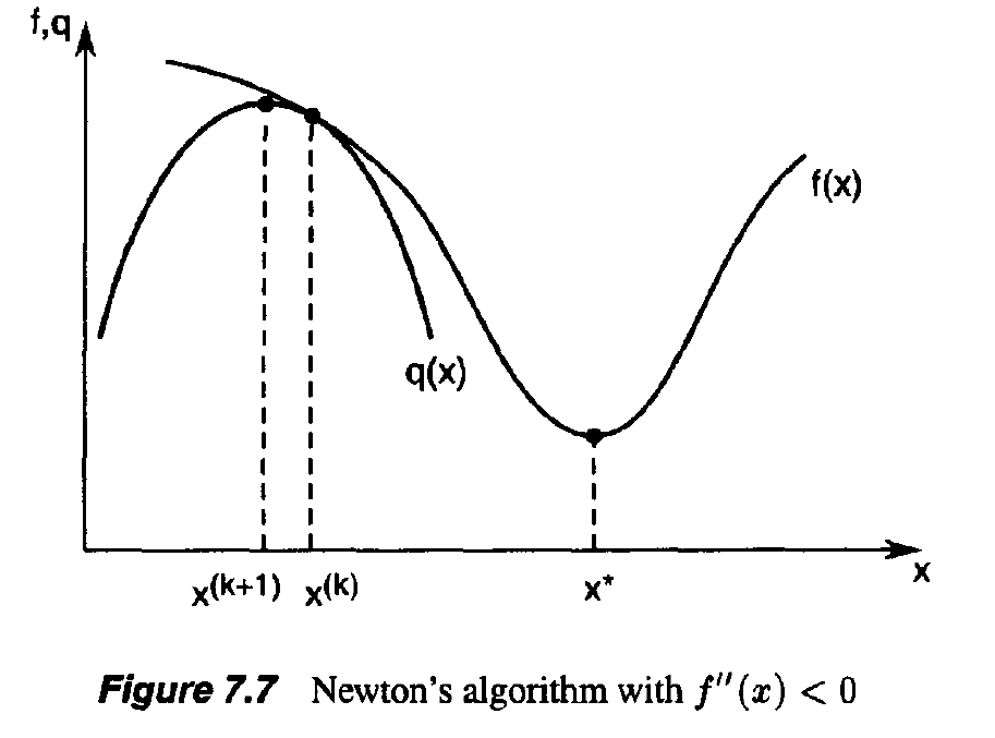
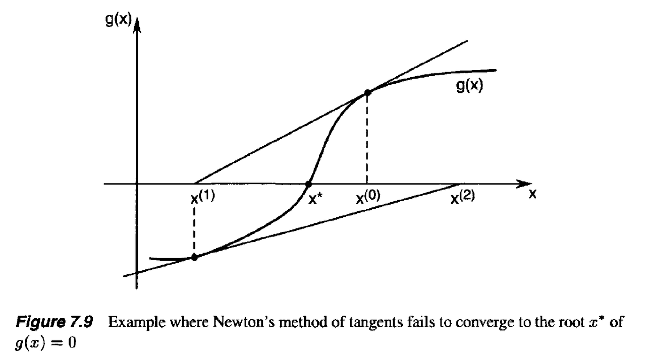
- Newton’s method works well if f “ ( x ) > 0 every where (see Figure 7.6). However, if f”(x) < 0 for some x, Newton’s method may fail to converge to the minimizer (see Figure 7.7).
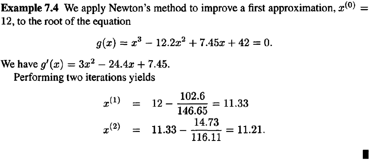
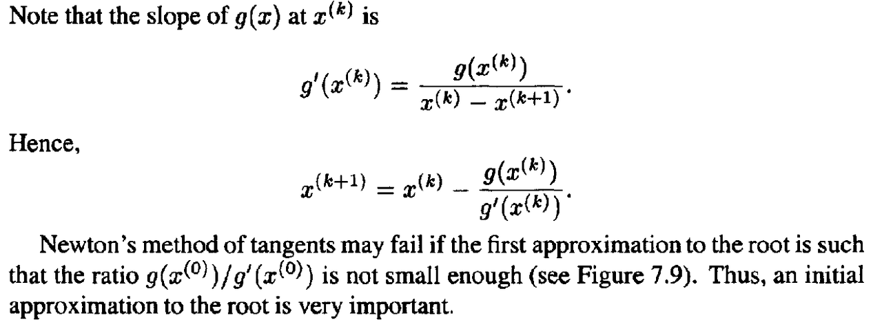
- Newton’s method can also be viewed as a way to drive the first derivative of f to zero. Indeed, if we set g(x) = f ‘ ( x ) , then we obtain a formula for iterative solution of the equation g(x) = 0:
Example 2
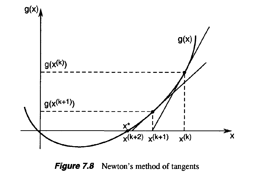
- Newton’s method for solving equations of the form g(x) = 0 is also referred to as Newton’s method of tangents.
- This name is easily justified if we look at a geometric interpretation of the method when applied to the solution of the equation g(x) = 0
- If we draw a tangent to g(x) at the given point $x^k$, then the tangent line intersects the x-axis at the point x^(k+1), which we expect to be closer to the root x* of g(x) = 0.
4. SECANT METHOD
- Newton’s method for minimizing f uses second derivatives of f:
- If the second derivative is not available, we may attempt to approximate it using first derivative information.
- In particular, we may approximate f”($x^k$} above with
- Using the above approximation of the second derivative, we obtain the algorithm:
- The above algorithm is called the secant method.
- Note that the algorithm requires two initial points to start it, which we denote x^(-1) and x^(0)
- The secant algorithm can be represented in the following equivalent form:
- Observe that, like Newton’s method, the secant method does not directly involve values of f($x^k$). Instead, it tries to drive the derivative f’ to zero.
- In fact, as we did for Newton’s method, we can interpret the secant method as an algorithm for solving equations of the form g(x) =Q.
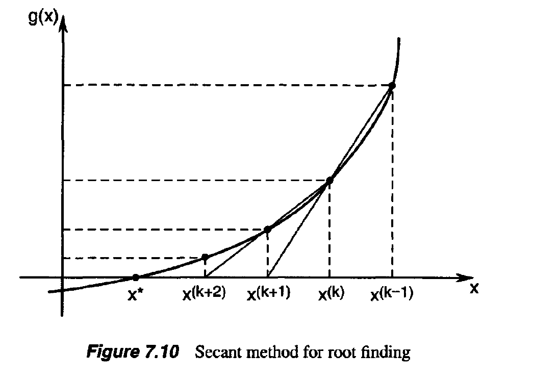
- Specifically, the secant algorithm for finding a root of the equation g(x) = 0 takes the form
- The secant method for root finding is illustrated in Figure 7.10 (compare this with Figure 7.8).
- Unlike Newton’s method, which uses the slope of g to determine the next point, the secant method uses the “secant” between the (k — l)st and kth points to determine the (k + l)st point.
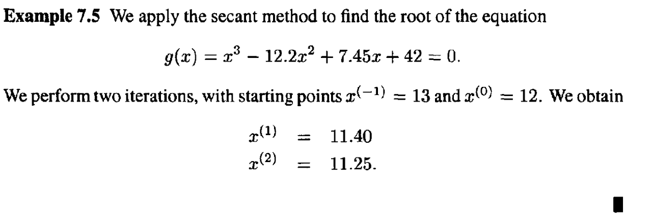
Example 1
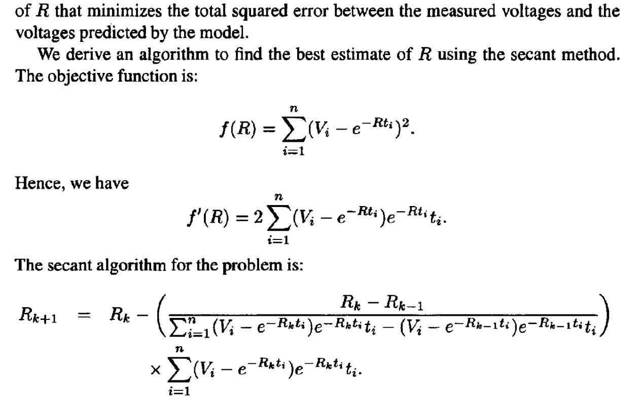
Example 2
5. REMARKS ON LINE SEARCH METHODS
- One-dimensional search methods play an important role in multidimensional optimization problems
- In particular, iterative algorithms for solving such optimization problems (to be discussed in the following chapters) typically involve a “line search” at every iteration.
- To be specific, let / : W1 -4 R be a function that we wish to minimize.
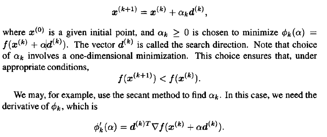
- Iterative algorithms for finding a minimizer of f are of the form:
- The above is obtained using the chain rule.
- Therefore, applying the secant method for the line search requires the gradient f.
- the initial line search point $x^k$ and the search direction $d^k$
- Of course, other one-dimensional search methods may be used for line search
Reference
Optimization method - Standford University
https://www.youtube.com/results?search_query=convex+function
1. GOLDEN SECTION SEARCH
- The search methods we discuss in this and the next section allow us to determine the minimizer of a function f : R —> R over a closed interval, say [$a_o$, $b_o$]
- The only property that we assume of the objective function f is that it is unimodal(단 한가지의 모델)
- which means that f has only one local minimizer
- The methods we discuss are based on evaluating the objective function at different points in the interval [$a_o$, $b_o$]
- We choose these points in such a way that an approximation to the minimizer of / may be achieved in as few evaluations as possible.
- Our goal is to progressively narrow the range until the minimizer is “boxed in” with sufficient accuracy.
- Consider a unimodal function / of one variable and the interval [$a_o$, $b_o$].
- If we evaluate / at only one intermediate point of the interval, we cannot narrow the range within which we know the minimizer is located.
- We have to evaluate f at two intermediate points
- We choose the intermediate points in such a way that the reduction in the range is symmetric, in the sense that:
- We then evaluate f at the intermediate points
-
If f($a_1$) < f($a_2$), then the minimizer must lie in the range [$a_0$, $b_1$]. If, on the other hand,f($a_1$) >= f($a_2$), then the minimizer is located in the range [$a_1$, $b_0$]
- Starting with the reduced range of uncertainty we can repeat the process and similarly find two new points, say $a_2$ and $b_2$ using the same value of p < 1/2
- However, we would like to minimize the number of the objective function evaluations while reducing the width of the uncertainty interval.
- Suppose, for example, that f($a_1$) < f($b_1$), as in Figure 7.3.
- Because $a_1$ is already in the uncertainty interval and f ( $a_1$ ) is already known, we can make $a_1$ coincide with $b_2$
- Thus, only one new evaluation of f at $a_2$ would be necessary
- To find the value of p that results in only one new evaluation of f
- Without loss of generality, imagine that the original range [$a_0$, $b_0$] is of unit length.
- Thus, dividing a range in the ratio of p to 1 — p has the effect that the ratio of the shorter segment to the longer equals the ratio of the longer to the sum of the two.
- This rule was referred to by ancient Greek geometers as the Golden Section.
- Using this Golden Section rule means that at every stage of the uncertainty range reduction (except the first one), the objective function f need only be evaluated at one new point.
- The uncertainty range is reduced by the ratio 1 — p = 0.61803 at every stage.
- Hence, N steps of reduction using the Golden Section method reduces the range by the factor
Example
2. FIBONACCI SEARCH
- Recall that the Golden Section method uses the same value of p throughout
- Suppose now that we are allowed to vary the value p from stage to stage, so that at the k th stage in the reduction process we use a value $p_k$, at the next stage we use a value p(k+1), and so on.
- As in the Golden Section search, our goal is to select successive values of $p_k$, 0 < $P_k$ < 1/2, such that only one new function evaluation is required at each stage.
- From Figure 7.5, we see that it is sufficient to choose the $p_k$ such that:
- There are many sequences $p_1$,$p_2$, • • • that satisfy the above law of formation, and the condition that 0 < $p_k$ < 1/2.
- Suppose that we are given a sequence $p_1$,$p_2$, - - • satisfying the above conditions, and we use this sequence in our search algorithm.
- Then, after N iterations of the algorithm, the uncertainty range is reduced by a factor of
- Depending on the sequence $p_1$,$p_2$,…, we get a different reduction factor.
- The natural question is as follows: What sequence $p_1$,$p_2$,… minimizes the above reduction factor?
- This problem is a constrained optimization problem that can be formally stated:
- Before we give the solution to the above optimization problem, we first need to introduce the Fibonacci sequence, FI,F2,F3, — This sequence is defined as follows. First, let F(-1) = 0 and F(0) = 1 by convention. Then, for k > 0,
- where the $F_k$ are the elements of the Fibonacci sequence.
- The resulting algorithm is called the Fibonacci search method.
- In the Fibonacci search method, the uncertainty range is reduced by the factor:
- Because the Fibonacci method uses the optimal values of $p_1$,$p_2$, • • •» the above reduction factor is less than that of the Golden Section method.
- In other words, the Fibonacci method is better than the Golden Section method in that it gives a smaller final uncertainty range.
- We point out that there is an anomaly in the final iteration of the Fibonacci search method, because:
- Recall that we need two intermediate points at each stage, one that comes from a previous iteration and another that is a new evaluation point.
- However, with $p_N$ = 1/2, the two intermediate points coincide in the middle of the uncertainty interval, and therefore we cannot further reduce the uncertainty range.
- To get around, this problem, we perform the new evaluation for the last iteration using $p_N$ = 1/2 - ε, where ε is the small number
- In other words, the new evaluation point is just to the left or right of the midpoint of the uncertainty interval.
- This modification to the Fibonacci method is, of course, of no significant practical consequence
- As a result of the above modification, the reduction in the uncertainty range at the last iteration may be either
- depending on which of the two points has the smaller objective function value.
- Therefore, in the worst case, the reduction factor in the uncertainty range for the Fibonacci method is
Example
3. NEWTON’S METHOD
- Suppose again that we are confronted(降临于) with the problem of minimizing a function f of a single real variable x.
- We assume now that at each measurement point $x^k$ we can calculate f($x^k$), f’’($x^k$}, and f’’’($x^k$). We can fit a quadratic function through $x^k$ that matches its first and second derivatives with that of the function f.
- This quadratic has the form :
Example 1
- Newton’s method works well if f “ ( x ) > 0 every where (see Figure 7.6). However, if f”(x) < 0 for some x, Newton’s method may fail to converge to the minimizer (see Figure 7.7).
- Newton’s method can also be viewed as a way to drive the first derivative of f to zero. Indeed, if we set g(x) = f ‘ ( x ) , then we obtain a formula for iterative solution of the equation g(x) = 0:
Example 2
- Newton’s method for solving equations of the form g(x) = 0 is also referred to as Newton’s method of tangents.
- This name is easily justified if we look at a geometric interpretation of the method when applied to the solution of the equation g(x) = 0
- If we draw a tangent to g(x) at the given point $x^k$, then the tangent line intersects the x-axis at the point x^(k+1), which we expect to be closer to the root x* of g(x) = 0.
4. SECANT METHOD
- Newton’s method for minimizing f uses second derivatives of f:
- If the second derivative is not available, we may attempt to approximate it using first derivative information.
- In particular, we may approximate f”($x^k$} above with
- Using the above approximation of the second derivative, we obtain the algorithm:
- The above algorithm is called the secant method.
- Note that the algorithm requires two initial points to start it, which we denote x^(-1) and x^(0)
- The secant algorithm can be represented in the following equivalent form:
- Observe that, like Newton’s method, the secant method does not directly involve values of f($x^k$). Instead, it tries to drive the derivative f’ to zero.
- In fact, as we did for Newton’s method, we can interpret the secant method as an algorithm for solving equations of the form g(x) =Q.
- Specifically, the secant algorithm for finding a root of the equation g(x) = 0 takes the form
- The secant method for root finding is illustrated in Figure 7.10 (compare this with Figure 7.8).
- Unlike Newton’s method, which uses the slope of g to determine the next point, the secant method uses the “secant” between the (k — l)st and kth points to determine the (k + l)st point.
Example 1
Example 2
5. REMARKS ON LINE SEARCH METHODS
- One-dimensional search methods play an important role in multidimensional optimization problems
- In particular, iterative algorithms for solving such optimization problems (to be discussed in the following chapters) typically involve a “line search” at every iteration.
- To be specific, let / : W1 -4 R be a function that we wish to minimize.
- Iterative algorithms for finding a minimizer of f are of the form:
- The above is obtained using the chain rule.
- Therefore, applying the secant method for the line search requires the gradient f.
- the initial line search point $x^k$ and the search direction $d^k$
- Of course, other one-dimensional search methods may be used for line search
Reference
Optimization method - Standford University
https://www.youtube.com/results?search_query=convex+function
















Comments