14. BREAST CANCER CLASSIFICATION
14 Sep 2019 | Python
PROBLEM STATEMENT
- Predicting if the cancer diagnosis is benign or malignant based on several observations/features
- 30 features are used, examples:
- radius (mean of distances from center to points on the perimeter 주의)
- texture (standard deviation of gray-scale values)
- perimeter(外缘)
- area
- smoothness (local variation in radius lengths)
- compactness (perimeter^2 / area - 1.0)
- concavity (severity of concave(凹面的) portions of the contour)
- concave points (number of concave portions of the contour)
- symmetry
- fractal(分形) dimension (“coastline approximation” - 1)
- Datasets are linearly separable using all 30 input features
- Number of Instances: 569
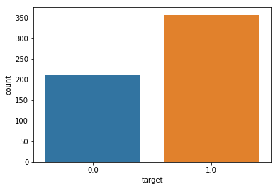
- Class Distribution: 212 Malignant(恶性的), 357 Benign(善良的;)
- Target Class
- Malignant
- Benign
- https://archive.ics.uci.edu/ml/datasets/Breast+Cancer+Wisconsin+(Diagnostic)
Step 1 Importing data
# import libraries
import pandas as pd # Import Pandas for data manipulation using dataframes
import numpy as np # Import Numpy for data statistical analysis
import matplotlib.pyplot as plt # Import matplotlib for data visualisation
import seaborn as sns # Statistical data visualization
# %matplotlib inline
# Import Cancer data drom the Sklearn library
from sklearn.datasets import load_breast_cancer
cancer = load_breast_cancer()
cancer
{'data': array([[1.799e+01, 1.038e+01, 1.228e+02, ..., 2.654e-01, 4.601e-01,
         1.189e-01],
        [2.057e+01, 1.777e+01, 1.329e+02, ..., 1.860e-01, 2.750e-01,
         8.902e-02],
        [1.969e+01, 2.125e+01, 1.300e+02, ..., 2.430e-01, 3.613e-01,
         8.758e-02],
        ...,
        [1.660e+01, 2.808e+01, 1.083e+02, ..., 1.418e-01, 2.218e-01,
         7.820e-02],
        [2.060e+01, 2.933e+01, 1.401e+02, ..., 2.650e-01, 4.087e-01,
         1.240e-01],
        [7.760e+00, 2.454e+01, 4.792e+01, ..., 0.000e+00, 2.871e-01,
         7.039e-02]]),
 'target': array([0, 0, 0, 0, 0, 0, 0, 0, 0, 0, 0, 0, 0, 0, 0, 0, 0, 0, 0, 1, 1, 1,
        0, 0, 0, 0, 0, 0, 0, 0, 0, 0, 0, 0, 0, 0, 0, 1, 0, 0, 0, 0, 0, 0,
        0, 0, 1, 0, 1, 1, 1, 1, 1, 0, 0, 1, 0, 0, 1, 1, 1, 1, 0, 1, 0, 0,
        1, 1, 1, 1, 0, 1, 0, 0, 1, 0, 1, 0, 0, 1, 1, 1, 0, 0, 1, 0, 0, 0,
        1, 1, 1, 0, 1, 1, 0, 0, 1, 1, 1, 0, 0, 1, 1, 1, 1, 0, 1, 1, 0, 1,
        1, 1, 1, 1, 1, 1, 1, 0, 0, 0, 1, 0, 0, 1, 1, 1, 0, 0, 1, 0, 1, 0,
        0, 1, 0, 0, 1, 1, 0, 1, 1, 0, 1, 1, 1, 1, 0, 1, 1, 1, 1, 1, 1, 1,
        1, 1, 0, 1, 1, 1, 1, 0, 0, 1, 0, 1, 1, 0, 0, 1, 1, 0, 0, 1, 1, 1,
        1, 0, 1, 1, 0, 0, 0, 1, 0, 1, 0, 1, 1, 1, 0, 1, 1, 0, 0, 1, 0, 0,
        0, 0, 1, 0, 0, 0, 1, 0, 1, 0, 1, 1, 0, 1, 0, 0, 0, 0, 1, 1, 0, 0,
        1, 1, 1, 0, 1, 1, 1, 1, 1, 0, 0, 1, 1, 0, 1, 1, 0, 0, 1, 0, 1, 1,
        1, 1, 0, 1, 1, 1, 1, 1, 0, 1, 0, 0, 0, 0, 0, 0, 0, 0, 0, 0, 0, 0,
        0, 0, 1, 1, 1, 1, 1, 1, 0, 1, 0, 1, 1, 0, 1, 1, 0, 1, 0, 0, 1, 1,
        1, 1, 1, 1, 1, 1, 1, 1, 1, 1, 1, 0, 1, 1, 0, 1, 0, 1, 1, 1, 1, 1,
        1, 1, 1, 1, 1, 1, 1, 1, 1, 0, 1, 1, 1, 0, 1, 0, 1, 1, 1, 1, 0, 0,
        0, 1, 1, 1, 1, 0, 1, 0, 1, 0, 1, 1, 1, 0, 1, 1, 1, 1, 1, 1, 1, 0,
        0, 0, 1, 1, 1, 1, 1, 1, 1, 1, 1, 1, 1, 0, 0, 1, 0, 0, 0, 1, 0, 0,
        1, 1, 1, 1, 1, 0, 1, 1, 1, 1, 1, 0, 1, 1, 1, 0, 1, 1, 0, 0, 1, 1,
        1, 1, 1, 1, 0, 1, 1, 1, 1, 1, 1, 1, 0, 1, 1, 1, 1, 1, 0, 1, 1, 0,
        1, 1, 1, 1, 1, 1, 1, 1, 1, 1, 1, 1, 0, 1, 0, 0, 1, 0, 1, 1, 1, 1,
        1, 0, 1, 1, 0, 1, 0, 1, 1, 0, 1, 0, 1, 1, 1, 1, 1, 1, 1, 1, 0, 0,
        1, 1, 1, 1, 1, 1, 0, 1, 1, 1, 1, 1, 1, 1, 1, 1, 1, 0, 1, 1, 1, 1,
        1, 1, 1, 0, 1, 0, 1, 1, 0, 1, 1, 1, 1, 1, 0, 0, 1, 0, 1, 0, 1, 1,
        1, 1, 1, 0, 1, 1, 0, 1, 0, 1, 0, 0, 1, 1, 1, 0, 1, 1, 1, 1, 1, 1,
        1, 1, 1, 1, 1, 0, 1, 0, 0, 1, 1, 1, 1, 1, 1, 1, 1, 1, 1, 1, 1, 1,
        1, 1, 1, 1, 1, 1, 1, 1, 1, 1, 1, 1, 0, 0, 0, 0, 0, 0, 1]),
cancer.keys()
# dict_keys(['data', 'target', 'target_names', 'DESCR', 'feature_names'])
print(cancer['DESCR'])
Breast Cancer Wisconsin (Diagnostic) Database
=============================================

Notes
-----
Data Set Characteristics:
    :Number of Instances: 569

    :Number of Attributes: 30 numeric, predictive attributes and the class

    :Attribute Information:
        - radius (mean of distances from center to points on the perimeter)
        - texture (standard deviation of gray-scale values)
        - perimeter
        - area
        - smoothness (local variation in radius lengths)
        - compactness (perimeter^2 / area - 1.0)
        - concavity (severity of concave portions of the contour)
        - concave points (number of concave portions of the contour)
        - symmetry
        - fractal dimension ("coastline approximation" - 1)

        The mean, standard error, and "worst" or largest (mean of the three
        largest values) of these features were computed for each image,
        resulting in 30 features.  For instance, field 3 is Mean Radius, field
        13 is Radius SE, field 23 is Worst Radius.

        - class:
                - WDBC-Malignant
                - WDBC-Benign

    :Summary Statistics:

    ===================================== ====== ======
                                           Min    Max
    ===================================== ====== ======
    radius (mean):                        6.981  28.11
    texture (mean):                       9.71   39.28
    perimeter (mean):                     43.79  188.5
    area (mean):                          143.5  2501.0
    smoothness (mean):                    0.053  0.163
    compactness (mean):                   0.019  0.345
    concavity (mean):                     0.0    0.427
    concave points (mean):                0.0    0.201
    symmetry (mean):                      0.106  0.304
    fractal dimension (mean):             0.05   0.097
    radius (standard error):              0.112  2.873
    texture (standard error):             0.36   4.885
    perimeter (standard error):           0.757  21.98
    area (standard error):                6.802  542.2
    smoothness (standard error):          0.002  0.031
    compactness (standard error):         0.002  0.135
    concavity (standard error):           0.0    0.396
    concave points (standard error):      0.0    0.053
    symmetry (standard error):            0.008  0.079
    fractal dimension (standard error):   0.001  0.03
    radius (worst):                       7.93   36.04
    texture (worst):                      12.02  49.54
    perimeter (worst):                    50.41  251.2
    area (worst):                         185.2  4254.0
    smoothness (worst):                   0.071  0.223
    compactness (worst):                  0.027  1.058
    concavity (worst):                    0.0    1.252
    concave points (worst):               0.0    0.291
    symmetry (worst):                     0.156  0.664
    fractal dimension (worst):            0.055  0.208
    ===================================== ====== ======

    :Missing Attribute Values: None

    :Class Distribution: 212 - Malignant, 357 - Benign

    :Creator:  Dr. William H. Wolberg, W. Nick Street, Olvi L. Mangasarian

    :Donor: Nick Street

    :Date: November, 1995

This is a copy of UCI ML Breast Cancer Wisconsin (Diagnostic) datasets.
https://goo.gl/U2Uwz2

Features are computed from a digitized image of a fine needle
aspirate (FNA) of a breast mass.  They describe
characteristics of the cell nuclei present in the image.

Separating plane described above was obtained using
Multisurface Method-Tree (MSM-T) [K. P. Bennett, "Decision Tree
Construction Via Linear Programming." Proceedings of the 4th
Midwest Artificial Intelligence and Cognitive Science Society,
pp. 97-101, 1992], a classification method which uses linear
programming to construct a decision tree.  Relevant features
were selected using an exhaustive search in the space of 1-4
features and 1-3 separating planes.

The actual linear program used to obtain the separating plane
in the 3-dimensional space is that described in:
[K. P. Bennett and O. L. Mangasarian: "Robust Linear
Programming Discrimination of Two Linearly Inseparable Sets",
Optimization Methods and Software 1, 1992, 23-34].

This database is also available through the UW CS ftp server:

ftp ftp.cs.wisc.edu
cd math-prog/cpo-dataset/machine-learn/WDBC/

References
----------
   - W.N. Street, W.H. Wolberg and O.L. Mangasarian. Nuclear feature extraction
     for breast tumor diagnosis. IS&T/SPIE 1993 International Symposium on
     Electronic Imaging: Science and Technology, volume 1905, pages 861-870,
     San Jose, CA, 1993.
   - O.L. Mangasarian, W.N. Street and W.H. Wolberg. Breast cancer diagnosis and
     prognosis via linear programming. Operations Research, 43(4), pages 570-577,
     July-August 1995.
   - W.H. Wolberg, W.N. Street, and O.L. Mangasarian. Machine learning techniques
     to diagnose breast cancer from fine-needle aspirates. Cancer Letters 77 (1994)
     163-171.
print(cancer['target_names'])
# Target name only have two malignant ,benign
# ['malignant' 'benign']
print(cancer['target'])
# 0 , 1 is the who has a cancer or not
print(cancer['target'])

# 0 , 1 is the who has a cancer or not

[0 0 0 0 0 0 0 0 0 0 0 0 0 0 0 0 0 0 0 1 1 1 0 0 0 0 0 0 0 0 0 0 0 0 0 0 0
 1 0 0 0 0 0 0 0 0 1 0 1 1 1 1 1 0 0 1 0 0 1 1 1 1 0 1 0 0 1 1 1 1 0 1 0 0
 1 0 1 0 0 1 1 1 0 0 1 0 0 0 1 1 1 0 1 1 0 0 1 1 1 0 0 1 1 1 1 0 1 1 0 1 1
 1 1 1 1 1 1 0 0 0 1 0 0 1 1 1 0 0 1 0 1 0 0 1 0 0 1 1 0 1 1 0 1 1 1 1 0 1
 1 1 1 1 1 1 1 1 0 1 1 1 1 0 0 1 0 1 1 0 0 1 1 0 0 1 1 1 1 0 1 1 0 0 0 1 0
 1 0 1 1 1 0 1 1 0 0 1 0 0 0 0 1 0 0 0 1 0 1 0 1 1 0 1 0 0 0 0 1 1 0 0 1 1
 1 0 1 1 1 1 1 0 0 1 1 0 1 1 0 0 1 0 1 1 1 1 0 1 1 1 1 1 0 1 0 0 0 0 0 0 0
 0 0 0 0 0 0 0 1 1 1 1 1 1 0 1 0 1 1 0 1 1 0 1 0 0 1 1 1 1 1 1 1 1 1 1 1 1
 1 0 1 1 0 1 0 1 1 1 1 1 1 1 1 1 1 1 1 1 1 0 1 1 1 0 1 0 1 1 1 1 0 0 0 1 1
 1 1 0 1 0 1 0 1 1 1 0 1 1 1 1 1 1 1 0 0 0 1 1 1 1 1 1 1 1 1 1 1 0 0 1 0 0
 0 1 0 0 1 1 1 1 1 0 1 1 1 1 1 0 1 1 1 0 1 1 0 0 1 1 1 1 1 1 0 1 1 1 1 1 1
 1 0 1 1 1 1 1 0 1 1 0 1 1 1 1 1 1 1 1 1 1 1 1 0 1 0 0 1 0 1 1 1 1 1 0 1 1
 0 1 0 1 1 0 1 0 1 1 1 1 1 1 1 1 0 0 1 1 1 1 1 1 0 1 1 1 1 1 1 1 1 1 1 0 1
 1 1 1 1 1 1 0 1 0 1 1 0 1 1 1 1 1 0 0 1 0 1 0 1 1 1 1 1 0 1 1 0 1 0 1 0 0
 1 1 1 0 1 1 1 1 1 1 1 1 1 1 1 0 1 0 0 1 1 1 1 1 1 1 1 1 1 1 1 1 1 1 1 1 1
 1 1 1 1 1 1 1 0 0 0 0 0 0 1]
print(cancer['feature_names'])
print(cancer['feature_names'])

['mean radius' 'mean texture' 'mean perimeter' 'mean area'
 'mean smoothness' 'mean compactness' 'mean concavity'
 'mean concave points' 'mean symmetry' 'mean fractal dimension'
 'radius error' 'texture error' 'perimeter error' 'area error'
 'smoothness error' 'compactness error' 'concavity error'
 'concave points error' 'symmetry error' 'fractal dimension error'
 'worst radius' 'worst texture' 'worst perimeter' 'worst area'
 'worst smoothness' 'worst compactness' 'worst concavity'
 'worst concave points' 'worst symmetry' 'worst fractal dimension']
print(cancer['data'])
[[1.799e+01 1.038e+01 1.228e+02 ... 2.654e-01 4.601e-01 1.189e-01]
 [2.057e+01 1.777e+01 1.329e+02 ... 1.860e-01 2.750e-01 8.902e-02]
 [1.969e+01 2.125e+01 1.300e+02 ... 2.430e-01 3.613e-01 8.758e-02]
 ...
 [1.660e+01 2.808e+01 1.083e+02 ... 1.418e-01 2.218e-01 7.820e-02]
 [2.060e+01 2.933e+01 1.401e+02 ... 2.650e-01 4.087e-01 1.240e-01]
 [7.760e+00 2.454e+01 4.792e+01 ... 0.000e+00 2.871e-01 7.039e-02]]
cancer['data'].shape #(569, 30)
#569 raw as data set, 30 is the 30 feature.
df_cancer = pd.DataFrame(np.c_[cancer['data'], cancer['target']], columns = np.append(cancer['feature_names'], ['target']))
# append two vecotr or two columns together. so we can have cancer name and target as well
# to make better dataframe, we use that.
# which means 30 columns all the data we had
# then can additional column withch the first column that includes a target data wich is kind of you know we can include all the trains the in put and output
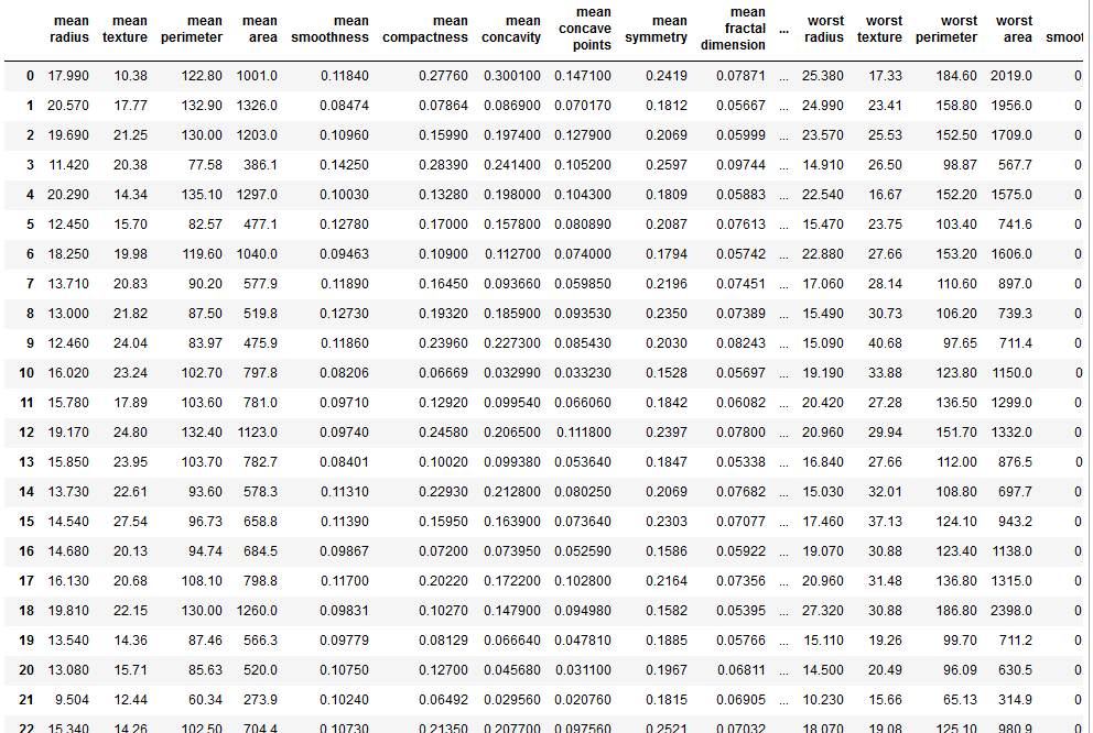
df_cancer.head()
#it showing our goal 'target'
x = np.array([1,2,3])
x.shape
# (3,)
Example = np.c_[np.array([1,2,3]), np.array([4,5,6])]
Example.shape
# (3, 2)
Step 2 Visualize data
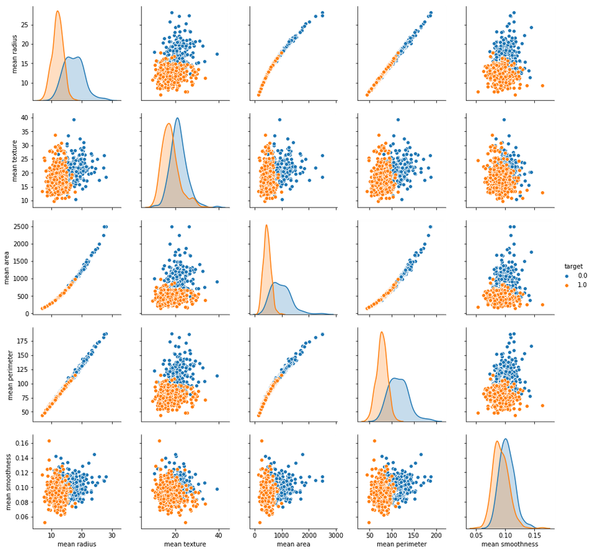
sns.pairplot(df_cancer, hue = 'target', vars = ['mean radius', 'mean texture', 'mean area', 'mean perimeter', 'mean smoothness'] )
# hue is the target of the data what we want to know about it
sns.countplot(df_cancer['target'], label = "Count")
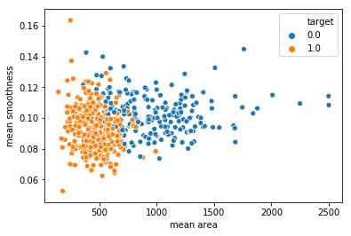
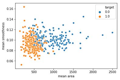
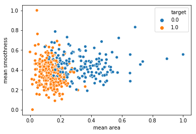
sns.scatterplot(x = 'mean area', y = 'mean smoothness', hue = 'target', data = df_cancer)
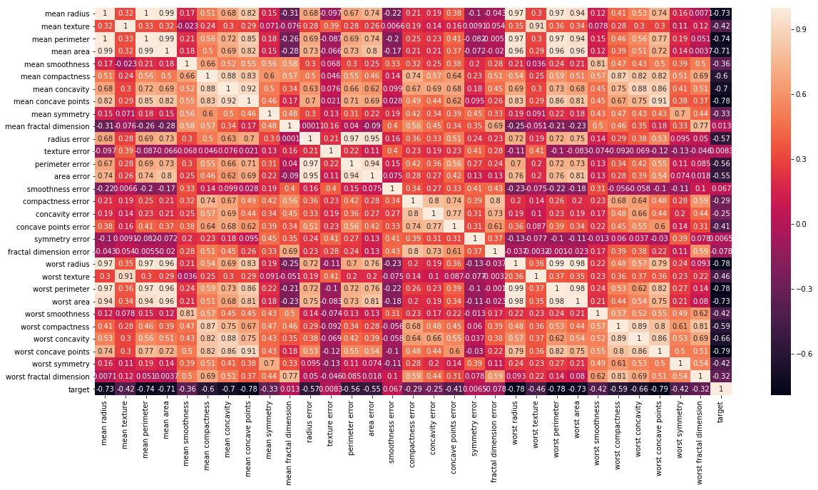
# Let's check the correlation between the variables
# Strong correlation between the mean radius and mean perimeter, mean area and mean primeter
plt.figure(figsize=(20,10))
sns.heatmap(df_cancer.corr(), annot=True)
Step 3 MODEL TRAINING (FINDING A PROBLEM SOLUTION)
# Let's drop the target label coloumns because we only need input data.
# target data is output we created
# axis=1 is we all delete data of target
X = df_cancer.drop(['target'],axis=1)
X
y = df_cancer['target']
y
0      0.0
1      0.0
2      0.0
3      0.0
4      0.0
5      0.0
6      0.0
7      0.0
8      0.0
9      0.0
10     0.0
11     0.0
12     0.0
13     0.0
14     0.0
15     0.0
16     0.0
17     0.0
18     0.0
19     1.0
20     1.0
21     1.0
22     0.0
23     0.0
24     0.0
25     0.0
26     0.0
27     0.0
28     0.0
29     0.0
      ...
from sklearn.model_selection import train_test_split

X_train, X_test, y_train, y_test = train_test_split(X, y, test_size = 0.20, random_state=5)

# random_state is the just seed
X_train.shape # (455, 30)
X_test.shape # (114, 30)
y_train.shape # (455,)
y_test.shape # (114,)

from sklearn.svm import SVC #support vector machine learning
from sklearn.metrics import classification_report, confusion_matrix
#confusion_matrix 오차 행렬
#matrix inside for moving foward

svc_model = SVC()
svc_model.fit(X_train, y_train)
from sklearn.svm import SVC #support vector machine learning
from sklearn.metrics import classification_report, confusion_matrix
#confusion_matrix 오차 행렬
#matrix inside for moving foward
svc_model = SVC()
svc_model.fit(X_train, y_train)
SVC(C=1.0, cache_size=200, class_weight=None, coef0=0.0,
decision_function_shape='ovr', degree=3, gamma='auto', kernel='rbf',
max_iter=-1, probability=False, random_state=None, shrinking=True,
tol=0.001, verbose=False)
Step 4 EVALUATING THE MODEL
y_predict = svc_model.predict(X_test)
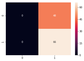
cm = confusion_matrix(y_test, y_predict)
sns.heatmap(cm, annot=True)
#annot is the showing the value
#showing that there is the a lot of the error
print(classification_report(y_test, y_predict))
precision    recall  f1-score   support

0.0       0.00      0.00      0.00        48
1.0       0.58      1.00      0.73        66

avg / total       0.34      0.58      0.42       114
Step 5 Improving the model
min_train = X_train.min()
#we are going to normalize the x-train. just get minimum value
min_train
mean radius                  6.981000
mean texture                 9.710000
mean perimeter              43.790000
mean area                  143.500000
mean smoothness              0.052630
mean compactness             0.019380
mean concavity               0.000000
mean concave points          0.000000
mean symmetry                0.106000
mean fractal dimension       0.049960
radius error                 0.111500
texture error                0.362100
perimeter error              0.757000
area error                   6.802000
smoothness error             0.001713
compactness error            0.002252
concavity error              0.000000
concave points error         0.000000
symmetry error               0.007882
fractal dimension error      0.000950
worst radius                 7.930000
worst texture               12.020000
worst perimeter             50.410000
worst area                 185.200000
worst smoothness             0.071170
worst compactness            0.027290
worst concavity              0.000000
worst concave points         0.000000
worst symmetry               0.156500
worst fractal dimension      0.055040
dtype: float64
range_train = (X_train - min_train).max()
#range to get maximum value of range_train
range_train
mean radius                  21.129000
mean texture                 29.570000
mean perimeter              144.710000
mean area                  2355.500000
mean smoothness               0.110770
mean compactness              0.326020
mean concavity                0.426800
mean concave points           0.201200
mean symmetry                 0.198000
mean fractal dimension        0.045790
radius error                  2.761500
texture error                 4.522900
perimeter error              21.223000
area error                  518.798000
smoothness error              0.029417
compactness error             0.133148
concavity error               0.396000
concave points error          0.052790
symmetry error                0.071068
fractal dimension error       0.028890
worst radius                 25.190000
worst texture                37.520000
worst perimeter             170.390000
worst area                 3246.800000
worst smoothness              0.129430
worst compactness             1.030710
worst concavity               1.105000
worst concave points          0.291000
worst symmetry                0.420900
worst fractal dimension       0.152460
dtype: float64
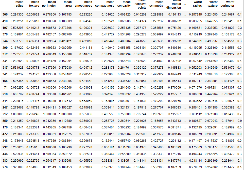
X_train_scaled = (X_train - min_train)/range_train
X_train_scaled
sns.scatterplot(x = X_train['mean area'], y = X_train['mean smoothness'], hue = y_train)
sns.scatterplot(x = X_train_scaled['mean area'], y = X_train_scaled['mean smoothness'], hue = y_train)
min_test = X_test.min()
range_test = (X_test - min_test).max()
X_test_scaled = (X_test - min_test)/range_test
from sklearn.svm import SVC
from sklearn.metrics import classification_report, confusion_matrix

svc_model = SVC()
svc_model.fit(X_train_scaled, y_train)

y_predict = svc_model.predict(X_test_scaled) # we use new data set. because the
# before normailzation, data is not good.
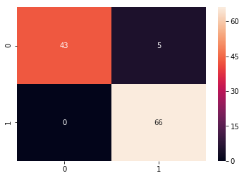
cm = confusion_matrix(y_test, y_predict)

sns.heatmap(cm,annot=True,fmt="d")
#fmt
print(classification_report(y_test,y_predict))
#to make classification_report.
#recall is how much well catch the true or not
#precision is how much good predict
         precision    recall  f1-score   support

0.0       1.00      0.90      0.95        48
1.0       0.93      1.00      0.96        66

avg / total       0.96      0.96      0.96       114
Step 5 Improving the model part 2
param_grid = {'C': [0.1, 1, 10, 100], 'gamma': [1, 0.1, 0.01, 0.001], 'kernel': ['rbf']}


#define our range.
# learning rate C and Gamma of blanket
#'C' parameter
# kernal is the basic function.
from sklearn.model_selection import GridSearchCV
#optimization for model

grid = GridSearchCV(SVC(),param_grid,refit=True,verbose=4)
# how many value we want to display that verbos , 4 ,5 what ever for our grid
# refit an estimator(추정법칙) using the best found parameters on the whole dataset
# verbose(冗长的)

grid.fit(X_train_scaled,y_train)
#seaching for best value of gamma and c
Fitting 3 folds for each of 16 candidates, totalling 48 fits
[CV] C=0.1, gamma=1, kernel=rbf ......................................
[CV]  C=0.1, gamma=1, kernel=rbf, score=0.9671052631578947, total=   0.0s
[CV] C=0.1, gamma=1, kernel=rbf ......................................
[CV]  C=0.1, gamma=1, kernel=rbf, score=0.9210526315789473, total=   0.0s
[CV] C=0.1, gamma=1, kernel=rbf ......................................
[CV]  C=0.1, gamma=1, kernel=rbf, score=0.9470198675496688, total=   0.0s
[CV] C=0.1, gamma=0.1, kernel=rbf ....................................
[CV]  C=0.1, gamma=0.1, kernel=rbf, score=0.9144736842105263, total=   0.0s
[CV] C=0.1, gamma=0.1, kernel=rbf ....................................
[CV]  C=0.1, gamma=0.1, kernel=rbf, score=0.8881578947368421, total=   0.0s
[CV] C=0.1, gamma=0.1, kernel=rbf ....................................
[CV]  C=0.1, gamma=0.1, kernel=rbf, score=0.8675496688741722, total=   0.0s
[CV] C=0.1, gamma=0.01, kernel=rbf ...................................
[CV]  C=0.1, gamma=0.01, kernel=rbf, score=0.6381578947368421, total=   0.0s
[CV] C=0.1, gamma=0.01, kernel=rbf ...................................
[CV]  C=0.1, gamma=0.01, kernel=rbf, score=0.6381578947368421, total=   0.0s
[CV] C=0.1, gamma=0.01, kernel=rbf ...................................
[CV]  C=0.1, gamma=0.01, kernel=rbf, score=0.6423841059602649, total=   0.0s
[CV] C=0.1, gamma=0.001, kernel=rbf ..................................
[CV]  C=0.1, gamma=0.001, kernel=rbf, score=0.6381578947368421, total=   0.0s
[CV] C=0.1, gamma=0.001, kernel=rbf ..................................
[CV]  C=0.1, gamma=0.001, kernel=rbf, score=0.6381578947368421, total=   0.0s
[CV] C=0.1, gamma=0.001, kernel=rbf ..................................
[CV]  C=0.1, gamma=0.001, kernel=rbf, score=0.6423841059602649, total=   0.0s
[CV] C=1, gamma=1, kernel=rbf ........................................
[CV]  C=1, gamma=1, kernel=rbf, score=0.993421052631579, total=   0.0s
[CV] C=1, gamma=1, kernel=rbf ........................................
[CV]  C=1, gamma=1, kernel=rbf, score=0.9473684210526315, total=   0.0s
[CV] C=1, gamma=1, kernel=rbf ........................................
[CV]  C=1, gamma=1, kernel=rbf, score=0.9801324503311258, total=   0.0s
[CV] C=1, gamma=0.1, kernel=rbf ......................................
[CV]  C=1, gamma=0.1, kernel=rbf, score=0.9736842105263158, total=   0.0s
[CV] C=1, gamma=0.1, kernel=rbf ......................................
[CV]  C=1, gamma=0.1, kernel=rbf, score=0.9276315789473685, total=   0.0s
[CV] C=1, gamma=0.1, kernel=rbf ......................................
[CV]  C=1, gamma=0.1, kernel=rbf, score=0.9403973509933775, total=   0.0s
[CV] C=1, gamma=0.01, kernel=rbf .....................................
[CV]  C=1, gamma=0.01, kernel=rbf, score=0.9144736842105263, total=   0.0s
grid.best_params_
# {'C': 10, 'gamma': 0.1, 'kernel': 'rbf'}
grid.best_estimator_
SVC(C=10, cache_size=200, class_weight=None, coef0=0.0,
  decision_function_shape='ovr', degree=3, gamma=0.1, kernel='rbf',
  max_iter=-1, probability=False, random_state=None, shrinking=True,
  tol=0.001, verbose=False)
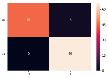
grid_predictions = grid.predict(X_test_scaled)
cm = confusion_matrix(y_test, grid_predictions)
sns.heatmap(cm, annot=True)
print(classification_report(y_test,grid_predictions))
precision    recall  f1-score   support

0.0       1.00      0.94      0.97        48
1.0       0.96      1.00      0.98        66

avg / total       0.97      0.97      0.97       114


Comments