3. Multi Armed Bandit
20 Sep 2019 | Reinforcement Learning
Multi Armed Bandit
- First saw in: bayesian Machine Learning(Probability Algorithm): A/B Testing (Ex. go to a Casino; choice between 3 slot machines)
- Each (for now) gives reward of 0 or 1
- win rate is unknown(Ex. Could be 0.1 0.3 0.5)
- Goal: Maximize our winnings
- Problem: can only discover best bandit by collecting data
- if we’re psychic, we could just play the bandit with highest win rate
- Balance explore(collectiong data) + exploit(playing “best-so-far” machines)
1.Traditional A/B Testing
- Predetermine # of times we need to play/collect data in order to establish statistical significance
- . # of times needed is dependent on numerous things like the difference between win rates of each bandit(but if we know that, we wouldn’t be doing this test, weird traditional statistics ideas)
- important rule: Don’t stop our test early. Even if we set N=1000, but after 500 trials, we discover 90% win-rate vs 10% win rate. we still may not stop
- Much different from Human behavior
- suppose we’re playing in a real casino, we get 2/3 on one bandit, 0/3 on the other.
- we have a strong urge to play the first Bandit
- we know “ as a data scientist” that 3 is a small sample size
- as a gambler we do not “feel” that way
- we look at ways to systematically make explore-exploit trade-off(explain upcoming next)
- better than these 2 suboptimal solutions: A/B testing, human emotion
2. Applications of Explore-Exploit
- Already discussed in bayesian Machine Learning
- if you don’t know let’s check it here
- Lots of scary math! How does it apply in the “real world”?
- the casino example seems contrived(预谋的)
- The explore-exploit dilemma(and the subsequent Algorithm which are intended to “solve” it) are one of the most, if not the most “real world” concepts in Machine Learning
- Almost every business and online entrepreneur can make use of them
3. Comparing things
- Quantitatively comparing things applies to almost any business(E.g. we are samsung, selling note8)
- we have 2 ads we really Like
- which one is better? the one more likely to lead the user to purchase the phone(naturally)
- Can measure the click-through rate(CTR) of each ad ( E.g. 10 Clicks/1000 impressions = 1 % CTR)
- How to measure the CTR? Do an Experiment
- Show the first ad to 1 million users and Show the second ad to 1 million users
- Calculate the CTRs and compare
- How do i know 1 million is the correct number?
4. The nature of Probability
- We would need an infinite number of samples to get an absolutely precise estimate of the CTR
- as we collect more samples, the confidence interval shrinks
- therefore, the more samples we collect, the better
- but, if one advertisement is better, that means the other is worse
- if i show the suboptimal(未达最佳标准的) ad 1 million times, i’ve wasted 1million impressions to get a suboptimal CTR
- my desire to show only the best advertisement(hence make more money) is fundamentally at odds with my desire to have an accurate CTR
- which is needed to know which advertisement is “best” in the first place
5. Who cares?
- apple is not the only company selling things
- almost every modern business uses online advertising
- but we don’t have to be one, we can simply be someone who owns a website
- Compare viewing time on old design vs new design
- is “Buy Now” button better at the top or bottom of sales pages?
- which “price ending” leads to the most conversions? ₩2000 vs ₩1999
- these are all the same problem numerically
- Note: Click Through and conversion rate is the same thing to us, just a generic “success rate”
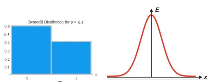
6. Gaussian vs Bernoulli
- Bernoulli good for measuring success rates
- Gaussian for Continuous variables
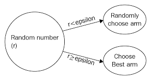
7. Epsilon-Greedy
- Solution to the explore-exploit dilemma
- Choose small number ε as Probability of exploration
- Typical values: 5%, 10%
p = random()
if p < eps:
  pull random arm
else:
  pull current-best  arm
- Eventually, we’ll discover which arm is the true best, since this allows us to update every arm’s estimate
- in the long run, allows us to explore each arm an infinite number of times
- Problem: we get to a point where we explore when we don’t need to
- For epsilon = 10%, we’ll continue to spend 10% of the time doing suboptimal things
- Could do A/B test at some Predetermined time, then set epsilon=0
- But we’ll learn better ways to adapt
8. Estimating Bandit Rewards
- Assuming bandit rewards are not just coin tosses.
- The best way to keep track of reward is General Method “Mean”
- Works for $ 1/0 $ too
\[P(k=1) = (#of1's)/(#of1's+#of0's) = (#of1's)/N\]
- P is Probability
- Need to keep Track of All X
- Can we be more efficient? YES!

- New mean can be calculated from old mean like that
- this “form” is very important to Reinforcement Learning
9. Let’s Recap how do this in supervised learning(Naive Bayes, Decision Trees, Neural Networks)
class Mymodel:
  def fit(x,y):
    # our job
  def Predict(x):
    # our job
- For example boilerplate
Xtrain, Ytrain, Xtest, Ytest  = get_data() # 1. Get data
model = Mymodel() # 2. Instantiate Model
model.fit(Xtrain,Ytrain)
model.socre(Xtest,Ytest)
10. Designing our bandit Program
- Since this is not Supervised learning, there is still a pattern to be followed
- Reminder: A “casino Machine” is just an analogy for real-life applications
- Serving advertisements you hope users will click on
- Testing different website design to see which keeps our users engaged longest
class MyAwesomeCasinoMachine:
  def pull():
    # simulates drawing from the true distribution
    # which we wouldnt know in "real life"
for t in range(max_iterations):
  # pick casino machine to play based on Algorithm
  # update Algorithm parameters
# plot useful info (ave reward, best machine, etc)
import numpy as np
import matplotlib.pyplot as plt

class bandit:
    """docstring for ."""

    def __init__(self, m):
        self.m = m
        self.mean = 0
        #the mean instance variable is our estimate of the bandit's mean
        self.N =0

    def pull(self):
        return np.random.randn() + self.m
    # the pull function which is simulates pulling the bandit's arm
    # every bandit's reward will be a gassium with unit variant


    def update(self, x):
        self.N +=1
        self.mean = (1 - 1.0/self.N)*self.mean + 1.0/self.N*x
    #Finally, we have the update function which takes an X, which is the latest sample recieved from the bandit
def run_experiment(m1,m2,m3,eps,N):
    # we are going to compare three different bandits
    bandits = [bandit(m1), bandit(m2),bandit(m3)]
    # Three difference means

    data = np.empty(N)

    for i in range(N):
        # epsilon greedy
        p = np.random.random()
        if p < eps:
            j = np.random.choice(3)
            # we choose a bandit at random
        else:
            j = np.argmax([b.mean for b in bandits])
            # we choose the bandit with the best current sample mean
        x=bandits[j].pull()
        bandits[j].update(x)
        # for the plot
        data[i] = x
    cumulative_average = np.cumsum(data) / (np.arange(N)+1)
    # cumulative_ averager after avery play

    #plt.plot(cumulative_average)
    plt.plot(cumulative_average)
    plt.plot(np.ones(N)*m1)
    plt.plot(np.ones(N)*m2)
    plt.plot(np.ones(N)*m3)
    plt.xscale('log')
    plt.show()

    for b in bandits:
        print (b.mean)

    return cumulative_average
if __name__ == '__main__':
    c_1 = run_experiment(1.0, 2.0, 3.0, 0.1, 100000)
    c_05 = run_experiment(1.0, 2.0, 3.0, 0.05, 100000)
    c_01 = run_experiment(1.0, 2.0, 3.0, 0.01, 100000)

    # log sacle plot
    plt.plot(c_1, label='eps = 0.1')
    plt.plot(c_05, label='eps = 0.05')
    plt.plot(c_01, label='eps = 0.01')
    plt.legend()
    plt.xscale('log')
    plt.show()

    # linear plot
    plt.plot(c_1, label='eps = 0.1')
    plt.plot(c_05, label='eps = 0.05')
    plt.plot(c_01, label='eps = 0.01')
    plt.legend()
    plt.show()
11.Optimistic Initial Values
- Another Simple way of solving the explore-exploit dilemma
- Suppose we know the true mean of each bandit is « 10
- pick a high ceiling as the initial mean estimate
- before we set initial mean to “0”, but this time we set initial value to “10”

- initial sample mean is “too good to be true “
- All collected data will cause it to go down
- if the true mean is 1, the sample mean will still approach 1 as I collect more samples
- All means will eventually settle into their true values(exploitation)
- Helps exploration as well
- if we haven’t explored a bandit, its mean will remain high, causing us to explore it more
- in the main loop: greedy strategy only
- but using optimistic means
- it make more looks like optimistic than “Mean”
Code
import numpy as np
import matplotlib.pyplot as plt
from Comparing_epsilons import run_experiment as run_experiment_eps

class bandit:
    """docstring for ."""

    def __init__(self, m, upper_limit = 10):
        self.m = m
        self.mean = upper_limit
        #the mean instance variable is our estimate of the bandit's mean
        self.N = 1

    def pull(self):
        return np.random.randn() + self.m
    # the pull function which is simulates pulling the bandit's arm
    # every bandit's reward will be a gassium with unit variant


    def update(self, x):
        self.N +=1
        self.mean = (1 - 1.0/self.N)*self.mean + 1.0/self.N*x

    #Finally, we have the update function which takes an X, which is the latest sample recieved from the bandit
def run_experiment(m1,m2,m3,N):
    # we are going to compare three different bandits
    bandits = [bandit(m1), bandit(m2),bandit(m3)]
    # Three difference means

    data = np.empty(N)

    for i in range(N):
        j = np.argmax([b.mean for b in bandits])
        # we choose the bandit with the best current sample mean
        x=bandits[j].pull()
        bandits[j].update(x)
        # for the plot
        data[i] = x
    cumulative_average = np.cumsum(data) / (np.arange(N)+1)
    # cumulative_ averager after avery play

    #plt.plot(cumulative_average)
    plt.plot(cumulative_average)
    plt.plot(np.ones(N)*m1)
    plt.plot(np.ones(N)*m2)
    plt.plot(np.ones(N)*m3)
    plt.xscale('log')
    plt.show()

    for b in bandits:
        print (b.mean)

    return cumulative_average
if __name__ == '__main__':
    c_1 = run_experiment_eps(1.0, 2.0, 3.0, 0.1, 100000)
    oiv = run_experiment(1.0, 2.0, 3.0, 100000)

    # log scale plot
    plt.plot(c_1, label='eps = 0.1')
    plt.plot(oiv, label='optimistic')
    plt.legend()
    plt.xscale('log')
    plt.show()

    # linear plot
    plt.plot(c_1, label='eps = 0.1')
    plt.plot(oiv, label='optimistic')
    plt.legend()
    plt.show()
Reference:
Artificial Intelligence Reinforcement Learning
Multi Armed Bandit
- First saw in: bayesian Machine Learning(Probability Algorithm): A/B Testing (Ex. go to a Casino; choice between 3 slot machines)
- Each (for now) gives reward of 0 or 1
- win rate is unknown(Ex. Could be 0.1 0.3 0.5)
- Goal: Maximize our winnings
- Problem: can only discover best bandit by collecting data
- if we’re psychic, we could just play the bandit with highest win rate
- Balance explore(collectiong data) + exploit(playing “best-so-far” machines)
1.Traditional A/B Testing
- Predetermine # of times we need to play/collect data in order to establish statistical significance
- . # of times needed is dependent on numerous things like the difference between win rates of each bandit(but if we know that, we wouldn’t be doing this test, weird traditional statistics ideas)
- important rule: Don’t stop our test early. Even if we set N=1000, but after 500 trials, we discover 90% win-rate vs 10% win rate. we still may not stop
- Much different from Human behavior
- suppose we’re playing in a real casino, we get 2/3 on one bandit, 0/3 on the other.
- we have a strong urge to play the first Bandit
- we know “ as a data scientist” that 3 is a small sample size
- as a gambler we do not “feel” that way
- we look at ways to systematically make explore-exploit trade-off(explain upcoming next)
- better than these 2 suboptimal solutions: A/B testing, human emotion
2. Applications of Explore-Exploit
- Already discussed in bayesian Machine Learning
- if you don’t know let’s check it here
- Lots of scary math! How does it apply in the “real world”?
- the casino example seems contrived(预谋的)
- The explore-exploit dilemma(and the subsequent Algorithm which are intended to “solve” it) are one of the most, if not the most “real world” concepts in Machine Learning
- Almost every business and online entrepreneur can make use of them
3. Comparing things
- Quantitatively comparing things applies to almost any business(E.g. we are samsung, selling note8)
- we have 2 ads we really Like
- which one is better? the one more likely to lead the user to purchase the phone(naturally)
- Can measure the click-through rate(CTR) of each ad ( E.g. 10 Clicks/1000 impressions = 1 % CTR)
- How to measure the CTR? Do an Experiment
- Show the first ad to 1 million users and Show the second ad to 1 million users
- Calculate the CTRs and compare
- How do i know 1 million is the correct number?
4. The nature of Probability
- We would need an infinite number of samples to get an absolutely precise estimate of the CTR
- as we collect more samples, the confidence interval shrinks
- therefore, the more samples we collect, the better
- but, if one advertisement is better, that means the other is worse
- if i show the suboptimal(未达最佳标准的) ad 1 million times, i’ve wasted 1million impressions to get a suboptimal CTR
- my desire to show only the best advertisement(hence make more money) is fundamentally at odds with my desire to have an accurate CTR
- which is needed to know which advertisement is “best” in the first place
5. Who cares?
- apple is not the only company selling things
- almost every modern business uses online advertising
- but we don’t have to be one, we can simply be someone who owns a website
- Compare viewing time on old design vs new design
- is “Buy Now” button better at the top or bottom of sales pages?
- which “price ending” leads to the most conversions? ₩2000 vs ₩1999
- these are all the same problem numerically
- Note: Click Through and conversion rate is the same thing to us, just a generic “success rate”
6. Gaussian vs Bernoulli
- Bernoulli good for measuring success rates
- Gaussian for Continuous variables
7. Epsilon-Greedy
- Solution to the explore-exploit dilemma
- Choose small number ε as Probability of exploration
- Typical values: 5%, 10%
p = random()
if p < eps:
pull random arm
else:
pull current-best arm
- Eventually, we’ll discover which arm is the true best, since this allows us to update every arm’s estimate
- in the long run, allows us to explore each arm an infinite number of times
- Problem: we get to a point where we explore when we don’t need to
- For epsilon = 10%, we’ll continue to spend 10% of the time doing suboptimal things
- Could do A/B test at some Predetermined time, then set epsilon=0
- But we’ll learn better ways to adapt
8. Estimating Bandit Rewards
- Assuming bandit rewards are not just coin tosses.
- The best way to keep track of reward is General Method “Mean”
- Works for $ 1/0 $ too
- P is Probability
- Need to keep Track of All X
- Can we be more efficient? YES!

- New mean can be calculated from old mean like that
- this “form” is very important to Reinforcement Learning
9. Let’s Recap how do this in supervised learning(Naive Bayes, Decision Trees, Neural Networks)
class Mymodel:
def fit(x,y):
# our job
def Predict(x):
# our job
- For example boilerplate
Xtrain, Ytrain, Xtest, Ytest = get_data() # 1. Get data
model = Mymodel() # 2. Instantiate Model
model.fit(Xtrain,Ytrain)
model.socre(Xtest,Ytest)
10. Designing our bandit Program
- Since this is not Supervised learning, there is still a pattern to be followed
- Reminder: A “casino Machine” is just an analogy for real-life applications
- Serving advertisements you hope users will click on
- Testing different website design to see which keeps our users engaged longest
class MyAwesomeCasinoMachine:
def pull():
# simulates drawing from the true distribution
# which we wouldnt know in "real life"
for t in range(max_iterations):
# pick casino machine to play based on Algorithm
# update Algorithm parameters
# plot useful info (ave reward, best machine, etc)
import numpy as np
import matplotlib.pyplot as plt
class bandit:
"""docstring for ."""
def __init__(self, m):
self.m = m
self.mean = 0
#the mean instance variable is our estimate of the bandit's mean
self.N =0
def pull(self):
return np.random.randn() + self.m
# the pull function which is simulates pulling the bandit's arm
# every bandit's reward will be a gassium with unit variant
def update(self, x):
self.N +=1
self.mean = (1 - 1.0/self.N)*self.mean + 1.0/self.N*x
#Finally, we have the update function which takes an X, which is the latest sample recieved from the bandit
def run_experiment(m1,m2,m3,eps,N):
# we are going to compare three different bandits
bandits = [bandit(m1), bandit(m2),bandit(m3)]
# Three difference means
data = np.empty(N)
for i in range(N):
# epsilon greedy
p = np.random.random()
if p < eps:
j = np.random.choice(3)
# we choose a bandit at random
else:
j = np.argmax([b.mean for b in bandits])
# we choose the bandit with the best current sample mean
x=bandits[j].pull()
bandits[j].update(x)
# for the plot
data[i] = x
cumulative_average = np.cumsum(data) / (np.arange(N)+1)
# cumulative_ averager after avery play
#plt.plot(cumulative_average)
plt.plot(cumulative_average)
plt.plot(np.ones(N)*m1)
plt.plot(np.ones(N)*m2)
plt.plot(np.ones(N)*m3)
plt.xscale('log')
plt.show()
for b in bandits:
print (b.mean)
return cumulative_average
if __name__ == '__main__':
c_1 = run_experiment(1.0, 2.0, 3.0, 0.1, 100000)
c_05 = run_experiment(1.0, 2.0, 3.0, 0.05, 100000)
c_01 = run_experiment(1.0, 2.0, 3.0, 0.01, 100000)
# log sacle plot
plt.plot(c_1, label='eps = 0.1')
plt.plot(c_05, label='eps = 0.05')
plt.plot(c_01, label='eps = 0.01')
plt.legend()
plt.xscale('log')
plt.show()
# linear plot
plt.plot(c_1, label='eps = 0.1')
plt.plot(c_05, label='eps = 0.05')
plt.plot(c_01, label='eps = 0.01')
plt.legend()
plt.show()
11.Optimistic Initial Values
- Another Simple way of solving the explore-exploit dilemma
- Suppose we know the true mean of each bandit is « 10
- pick a high ceiling as the initial mean estimate
- before we set initial mean to “0”, but this time we set initial value to “10”

- initial sample mean is “too good to be true “
- All collected data will cause it to go down
- if the true mean is 1, the sample mean will still approach 1 as I collect more samples
- All means will eventually settle into their true values(exploitation)
- Helps exploration as well
- if we haven’t explored a bandit, its mean will remain high, causing us to explore it more
- in the main loop: greedy strategy only
- but using optimistic means
- it make more looks like optimistic than “Mean”
Code
import numpy as np
import matplotlib.pyplot as plt
from Comparing_epsilons import run_experiment as run_experiment_eps
class bandit:
"""docstring for ."""
def __init__(self, m, upper_limit = 10):
self.m = m
self.mean = upper_limit
#the mean instance variable is our estimate of the bandit's mean
self.N = 1
def pull(self):
return np.random.randn() + self.m
# the pull function which is simulates pulling the bandit's arm
# every bandit's reward will be a gassium with unit variant
def update(self, x):
self.N +=1
self.mean = (1 - 1.0/self.N)*self.mean + 1.0/self.N*x
#Finally, we have the update function which takes an X, which is the latest sample recieved from the bandit
def run_experiment(m1,m2,m3,N):
# we are going to compare three different bandits
bandits = [bandit(m1), bandit(m2),bandit(m3)]
# Three difference means
data = np.empty(N)
for i in range(N):
j = np.argmax([b.mean for b in bandits])
# we choose the bandit with the best current sample mean
x=bandits[j].pull()
bandits[j].update(x)
# for the plot
data[i] = x
cumulative_average = np.cumsum(data) / (np.arange(N)+1)
# cumulative_ averager after avery play
#plt.plot(cumulative_average)
plt.plot(cumulative_average)
plt.plot(np.ones(N)*m1)
plt.plot(np.ones(N)*m2)
plt.plot(np.ones(N)*m3)
plt.xscale('log')
plt.show()
for b in bandits:
print (b.mean)
return cumulative_average
if __name__ == '__main__':
c_1 = run_experiment_eps(1.0, 2.0, 3.0, 0.1, 100000)
oiv = run_experiment(1.0, 2.0, 3.0, 100000)
# log scale plot
plt.plot(c_1, label='eps = 0.1')
plt.plot(oiv, label='optimistic')
plt.legend()
plt.xscale('log')
plt.show()
# linear plot
plt.plot(c_1, label='eps = 0.1')
plt.plot(oiv, label='optimistic')
plt.legend()
plt.show()
Reference:
Artificial Intelligence Reinforcement Learning


Comments