4. UCB1 and Bayesian Method
21 Sep 2019 | Reinforcement Learning
UCB1
- Another Method to Solve Explore-Exploit ( also from A/B Testing Classes)
- Idea: confidence bounds
- Intuitively, we know that sample mean from 10 samples is less accurate than a sample mean from 1000 samples
- Chefnoff Hoeffiding bound:

- Looks complicated, but leads to a simple algorithm

- square(2*ln(N)/N_j) <- “Choose” epsilon equal to this upper bound
- N = number of times i’ve played in total, N_j = number of times i’ve played bandit j
- How do we use this formular? Same as optimistic initial values Method
- just be greedy, but with respect to \(\ln{X}_{UCB-J}\)
- Key: ratio Between ln(N) and $N_j$
- if only $N_j$ is small, then upper bound is high
- if $N_j$ is large, upper bound is small
- ln(N) grow more slowly than N, so eventually all upper bounds will shrink
- by then we’ve collected lots of data, so it’s ok
- so we converge to purely greedy strategy
- ε-greedy는 추측값이나 불확실성과랑 관계없이 무조건 랜덤하게 실행하는 반면에 어떤 액션을 했을 때, 그 액션은 많이 해봤으니 어느정도 불확실할 것이라는 전재로 불확실성을 고려하여 액션을 취한다.)
- 즉 시간이 지날 수록 ln(N)의 값은 작아지는데, 많은 샘플들이 쌓이면 0으로 수렴함으로 결곡 적은 샘플을 가지고 있을때 취하는 액션들을 보정해준다고 보면 된다.
Code
import numpy as np
import matplotlib.pyplot as plt
from Comparing_epsilons import run_experiment as run_experiment_eps

class bandit:
    """docstring for ."""

    def __init__(self, m, upper_limit = 0):
        self.m = m
        self.mean = upper_limit
        #the mean instance variable is our estimate of the bandit's mean
        self.N = 1

    def pull(self):
        return np.random.randn() + self.m
    # the pull function which is simulates pulling the bandit's arm
    # every bandit's reward will be a gassium with unit variant


    def update(self, x):
        self.N +=1
        self.mean = (1 - 1.0/self.N)*self.mean + 1.0/self.N*x

    #Finally, we have the update function which takes an X, which is the latest sample recieved from the bandit
def ucb(mean, n, nj):
    if nj == 0:
        return float('inf') #infinity

    return mean + np.sqrt(2*np.log(n) / nj)
def run_experiment(m1, m2, m3, N):
    bandits = [bandit(m1), bandit(m2), bandit(m3)]

    data = np.empty(N)
    for i in range(N):
        j = np.argmax([ucb(b.mean, i+1, b.N) for b in bandits])
        x = bandits[j].pull()
        bandits[j].update(x)
        # for the plot
        data[i] = x
    cumulative_average = np.cumsum(data) / (np.arange(N) + 1)

  # for b in bandits:
  #   print("bandit nj:", b.N)

  # plot moving average ctr
    plt.plot(cumulative_average)
    plt.plot(np.ones(N)*m1)
    plt.plot(np.ones(N)*m2)
    plt.plot(np.ones(N)*m3)
    plt.xscale('log')
    plt.show()

  # for b in bandits:
  #   print(b.mean)
    return cumulative_average
if __name__ == '__main__':
    c_1 = run_experiment_eps(1.0, 2.0, 3.0, 0.1, 100000)
    ucb = run_experiment(1.0, 2.0, 3.0, 100000)

    # log scale plot
    plt.plot(c_1, label='eps = 0.1')
    plt.plot(ucb, label='ucb1')
    plt.legend()
    plt.xscale('log')
    plt.show()

    # linear plot
    plt.plot(c_1, label='eps = 0.1')
    plt.plot(ucb, label='ucb1')
    plt.legend()
    plt.show()
Bayesian Method
- thompson sampling(각 보상(reward) 분포의 파라미터 확률 변수를 보고 이 파라미터의 분포로 부터 무작위로 추출하여 해당 값에 대한 Reward 기대값이 가장 높은 기계를 선택한다. 그리고 나서 Bayesian 정리를 이용하여 기계에 대한 파라미터 분포를 업데이트 한다. Iteration을 하여 점점 높아지는 보상의 평균의 기계를 선택하게 된다.)
- Let’s think about confidence intervals again
- we know Intuitively that sample mean from 10 samples is less accurate than sample mean from 1000 samples
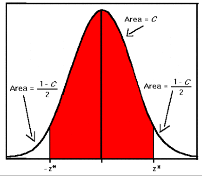
- Central Limit Theorem says that sample mean is approximately Gaussian
- Any Function of RVs is a RV(random Variable)

- Bayesian paradigm takes this a step further
- what if μ is Also a RV?
- Data is fixed; parameters are random
- we want to find the distribution of the parameter(入数) given the data
- should be more accurate than if did not have the data
- we call this the Posterior
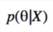
- Flip the Posterior to find it in terms of likelihood and prior
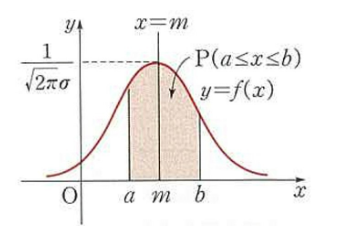
- Likelihood(연속 사건에서는 구간에 대한 추정은 가능하지만(PDF(Probability Density Function)), 특정사건에 대한 추정이 불가능할때 PDF에서 y값을 이용해서 P값을 구하겠다라는 것이다. 즉 0~100까지 있는 변수중에서 30을 뽑을 확률은 0이지만 likelihood로 보았을때에는 0.4인 것이다. 즉 세번 연속으로 뽑았을떄 2,49,20 이 나올 확룔은 0 X 0 X 0으로 0이지만, Likelihood에서는 0.4 x 0.2 x 0.01 = 0.008 이다.
- Disadvantage of Bayesian method: we must choose the prior
- Problem: Integral is usually intractable(很难处理的), we need “tricks” to solve this(만약 Bayesian으로 Posterior를 계산한다고 할 때, 각 항목이 일반적인 분포를 따르지 않늗다고 한다면(즉 들쑥 날쑥) 도출하는 방식이 매우 어렵기 때문에 Trick이 필요. 예로 입술에 빨간색이 뭍었을때 김치를 먹었는지 고추장을 먹었는지 예측할 수 있는 것이다.)
- special(likelihood,prior) pairs where we can easily solve this
- called conjugate priors(Likelihood가 특정 분포를 따른다고 할 때, Prior와 Posterior가 동일한 분포면 계산이 빨라진다.)
- Click-Through rate are like coin tosses; likelihood is bernoulli
- look up on wikipedia: what is conjugate prior for bernoulli likelihood? Beta (Posterior가 Likelihood의 특정분포를 따른다.)
- make sense; beta is in [0,1]
- Likelihood:

- Prior:

- combine likelihood and prior to solve for posterior:

- B(a,b) can be dropped (abosrbed into Normalization constant)
- Key: posterior takes the form of a beta distribution

-
New a,b : a’ = a + #1’s , b’ = b + #0’s
- script from A/B testing class: demonstrate to ourself how posterior is updated as we collect clicks/impressions(or heads/tails)
- we start with the priors $a_0$=1, $b_0$=0 (uniform distribution)
# From the course: Bayesin Machine Learning in Python: A/B Testing
# https://deeplearningcourses.com/c/bayesian-machine-learning-in-python-ab-testing
# https://www.udemy.com/bayesian-machine-learning-in-python-ab-testing
from __future__ import print_function, division
from builtins import range
# Note: you may need to update your version of future
# sudo pip install -U future


import numpy as np
import matplotlib.pyplot as plt
from scipy.stats import beta

def plot(a, b, trial, ctr):
  x = np.linspace(0, 1, 200)
  y = beta.pdf(x, a, b)
  mean = float(a) / (a + b)
  plt.plot(x, y)
  plt.title("Distributions after %s trials, true rate = %.1f, mean = %.2f" % (trial, ctr, mean))
  plt.show()

true_ctr = 0.3
a, b = 0, 1 # beta parameters
show = [0, 5, 10, 25, 50, 100, 200, 300, 500, 700, 1000, 1500]
for t in range(1501):
  coin_toss_result = (np.random.random() < true_ctr)
  if coin_toss_result:
    a += 1
  else:
    b += 1

  if t in show:
    plot(a, b, t+1, true_ctr)
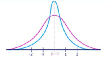
- Pattern: distribution of CTR gets skinnier/taller as we collect Data
- Because we’re becoming more confident in that estimate/variance decreases
- Natural way to represent confidence bounds
- is an instance of online learning
- distribution becomes more precise after every coin toss, not just after we collect all the data
- All the methods we’ll learn later (iterative update)
Application to the bandit Problem
- the key is sampling
- instead of upper confident bound like in UCB1, we take the argmax of our samples of each bandits
- Explore:
- Not much data; distributions are fat; can sample high values
- Exploit:
- Lots of data; distributions are skinny; will only sample near true mean
- The Bayesian Posterior automatically controls how much exploration/exploitation we do
- bayesian method(likelihood)를 이용하여 샘플이 많아 질수록 점점 뚜렷하게 잘 찾게 된다.
# From the course: Bayesin Machine Learning in Python: A/B Testing
# https://deeplearningcourses.com/c/bayesian-machine-learning-in-python-ab-testing
# https://www.udemy.com/bayesian-machine-learning-in-python-ab-testing
from __future__ import print_function, division
from builtins import range
# Note: you may need to update your version of future
# sudo pip install -U future


import matplotlib.pyplot as plt
import numpy as np
from scipy.stats import beta


NUM_TRIALS = 2000
BANDIT_PROBABILITIES = [0.2, 0.5, 0.75]


class Bandit(object):
  def __init__(self, p):
    self.p = p
    self.a = 1
    self.b = 1

  def pull(self):
    return np.random.random() < self.p

  def sample(self):
    return np.random.beta(self.a, self.b)

  def update(self, x):
    self.a += x
    self.b += 1 - x


def plot(bandits, trial):
  x = np.linspace(0, 1, 200)
  for b in bandits:
    y = beta.pdf(x, b.a, b.b)
    plt.plot(x, y, label="real p: %.4f" % b.p)
  plt.title("Bandit distributions after %s trials" % trial)
  plt.legend()
  plt.show()


def experiment():
  bandits = [Bandit(p) for p in BANDIT_PROBABILITIES]

  sample_points = [5,10,20,50,100,200,500,1000,1500,1999]
  for i in range(NUM_TRIALS):

    # take a sample from each bandit
    bestb = None
    maxsample = -1
    allsamples = [] # let's collect these just to print for debugging
    for b in bandits:
      sample = b.sample()
      allsamples.append("%.4f" % sample)
      if sample > maxsample:
        maxsample = sample
        bestb = b
    if i in sample_points:
      print("current samples: %s" % allsamples)
      plot(bandits, i)

    # pull the arm for the bandit with the largest sample
    x = bestb.pull()

    # update the distribution for the bandit whose arm we just pulled
    bestb.update(x)


if __name__ == "__main__":
  experiment()
참조) Gaussian Likelihood/Prior
- data likelihood is Gaussian
- we try to find μ only (also Gaussian)

- Work with precisions(inverse variance)
- Easier
- we’re looking for the update equations for m and λ
- Gaussian Posterior:

- Drop constant (constant wrt(with regard to)mu):

- collect like terms and ignore more constant:

- the form we are looking for :

- but this is what we just found
- Equate(同等看待)

Reference:
Artificial Intelligence Reinforcement Learning
UCB1
- Another Method to Solve Explore-Exploit ( also from A/B Testing Classes)
- Idea: confidence bounds
- Intuitively, we know that sample mean from 10 samples is less accurate than a sample mean from 1000 samples
- Chefnoff Hoeffiding bound:

- Looks complicated, but leads to a simple algorithm

- square(2*ln(N)/N_j) <- “Choose” epsilon equal to this upper bound
- N = number of times i’ve played in total, N_j = number of times i’ve played bandit j
- How do we use this formular? Same as optimistic initial values Method
- just be greedy, but with respect to \(\ln{X}_{UCB-J}\)
- Key: ratio Between ln(N) and $N_j$
- if only $N_j$ is small, then upper bound is high
- if $N_j$ is large, upper bound is small
- ln(N) grow more slowly than N, so eventually all upper bounds will shrink
- by then we’ve collected lots of data, so it’s ok
- so we converge to purely greedy strategy
- ε-greedy는 추측값이나 불확실성과랑 관계없이 무조건 랜덤하게 실행하는 반면에 어떤 액션을 했을 때, 그 액션은 많이 해봤으니 어느정도 불확실할 것이라는 전재로 불확실성을 고려하여 액션을 취한다.)
- 즉 시간이 지날 수록 ln(N)의 값은 작아지는데, 많은 샘플들이 쌓이면 0으로 수렴함으로 결곡 적은 샘플을 가지고 있을때 취하는 액션들을 보정해준다고 보면 된다.
Code
import numpy as np
import matplotlib.pyplot as plt
from Comparing_epsilons import run_experiment as run_experiment_eps
class bandit:
"""docstring for ."""
def __init__(self, m, upper_limit = 0):
self.m = m
self.mean = upper_limit
#the mean instance variable is our estimate of the bandit's mean
self.N = 1
def pull(self):
return np.random.randn() + self.m
# the pull function which is simulates pulling the bandit's arm
# every bandit's reward will be a gassium with unit variant
def update(self, x):
self.N +=1
self.mean = (1 - 1.0/self.N)*self.mean + 1.0/self.N*x
#Finally, we have the update function which takes an X, which is the latest sample recieved from the bandit
def ucb(mean, n, nj):
if nj == 0:
return float('inf') #infinity
return mean + np.sqrt(2*np.log(n) / nj)
def run_experiment(m1, m2, m3, N):
bandits = [bandit(m1), bandit(m2), bandit(m3)]
data = np.empty(N)
for i in range(N):
j = np.argmax([ucb(b.mean, i+1, b.N) for b in bandits])
x = bandits[j].pull()
bandits[j].update(x)
# for the plot
data[i] = x
cumulative_average = np.cumsum(data) / (np.arange(N) + 1)
# for b in bandits:
# print("bandit nj:", b.N)
# plot moving average ctr
plt.plot(cumulative_average)
plt.plot(np.ones(N)*m1)
plt.plot(np.ones(N)*m2)
plt.plot(np.ones(N)*m3)
plt.xscale('log')
plt.show()
# for b in bandits:
# print(b.mean)
return cumulative_average
if __name__ == '__main__':
c_1 = run_experiment_eps(1.0, 2.0, 3.0, 0.1, 100000)
ucb = run_experiment(1.0, 2.0, 3.0, 100000)
# log scale plot
plt.plot(c_1, label='eps = 0.1')
plt.plot(ucb, label='ucb1')
plt.legend()
plt.xscale('log')
plt.show()
# linear plot
plt.plot(c_1, label='eps = 0.1')
plt.plot(ucb, label='ucb1')
plt.legend()
plt.show()
Bayesian Method
- thompson sampling(각 보상(reward) 분포의 파라미터 확률 변수를 보고 이 파라미터의 분포로 부터 무작위로 추출하여 해당 값에 대한 Reward 기대값이 가장 높은 기계를 선택한다. 그리고 나서 Bayesian 정리를 이용하여 기계에 대한 파라미터 분포를 업데이트 한다. Iteration을 하여 점점 높아지는 보상의 평균의 기계를 선택하게 된다.)
- Let’s think about confidence intervals again
- we know Intuitively that sample mean from 10 samples is less accurate than sample mean from 1000 samples
- Central Limit Theorem says that sample mean is approximately Gaussian
- Any Function of RVs is a RV(random Variable)

- Bayesian paradigm takes this a step further
- what if μ is Also a RV?
- Data is fixed; parameters are random
- we want to find the distribution of the parameter(入数) given the data
- should be more accurate than if did not have the data
- we call this the Posterior

- Flip the Posterior to find it in terms of likelihood and prior

- Likelihood(연속 사건에서는 구간에 대한 추정은 가능하지만(PDF(Probability Density Function)), 특정사건에 대한 추정이 불가능할때 PDF에서 y값을 이용해서 P값을 구하겠다라는 것이다. 즉 0~100까지 있는 변수중에서 30을 뽑을 확률은 0이지만 likelihood로 보았을때에는 0.4인 것이다. 즉 세번 연속으로 뽑았을떄 2,49,20 이 나올 확룔은 0 X 0 X 0으로 0이지만, Likelihood에서는 0.4 x 0.2 x 0.01 = 0.008 이다.
- Disadvantage of Bayesian method: we must choose the prior
- Problem: Integral is usually intractable(很难处理的), we need “tricks” to solve this(만약 Bayesian으로 Posterior를 계산한다고 할 때, 각 항목이 일반적인 분포를 따르지 않늗다고 한다면(즉 들쑥 날쑥) 도출하는 방식이 매우 어렵기 때문에 Trick이 필요. 예로 입술에 빨간색이 뭍었을때 김치를 먹었는지 고추장을 먹었는지 예측할 수 있는 것이다.)
- special(likelihood,prior) pairs where we can easily solve this
- called conjugate priors(Likelihood가 특정 분포를 따른다고 할 때, Prior와 Posterior가 동일한 분포면 계산이 빨라진다.)
- Click-Through rate are like coin tosses; likelihood is bernoulli
- look up on wikipedia: what is conjugate prior for bernoulli likelihood? Beta (Posterior가 Likelihood의 특정분포를 따른다.)
- make sense; beta is in [0,1]
- Likelihood:

- Prior:

- combine likelihood and prior to solve for posterior:

- B(a,b) can be dropped (abosrbed into Normalization constant)
- Key: posterior takes the form of a beta distribution

-
New a,b : a’ = a + #1’s , b’ = b + #0’s
- script from A/B testing class: demonstrate to ourself how posterior is updated as we collect clicks/impressions(or heads/tails)
- we start with the priors $a_0$=1, $b_0$=0 (uniform distribution)
# From the course: Bayesin Machine Learning in Python: A/B Testing
# https://deeplearningcourses.com/c/bayesian-machine-learning-in-python-ab-testing
# https://www.udemy.com/bayesian-machine-learning-in-python-ab-testing
from __future__ import print_function, division
from builtins import range
# Note: you may need to update your version of future
# sudo pip install -U future
import numpy as np
import matplotlib.pyplot as plt
from scipy.stats import beta
def plot(a, b, trial, ctr):
x = np.linspace(0, 1, 200)
y = beta.pdf(x, a, b)
mean = float(a) / (a + b)
plt.plot(x, y)
plt.title("Distributions after %s trials, true rate = %.1f, mean = %.2f" % (trial, ctr, mean))
plt.show()
true_ctr = 0.3
a, b = 0, 1 # beta parameters
show = [0, 5, 10, 25, 50, 100, 200, 300, 500, 700, 1000, 1500]
for t in range(1501):
coin_toss_result = (np.random.random() < true_ctr)
if coin_toss_result:
a += 1
else:
b += 1
if t in show:
plot(a, b, t+1, true_ctr)
- Pattern: distribution of CTR gets skinnier/taller as we collect Data
- Because we’re becoming more confident in that estimate/variance decreases
- Natural way to represent confidence bounds
- is an instance of online learning
- distribution becomes more precise after every coin toss, not just after we collect all the data
- All the methods we’ll learn later (iterative update)
Application to the bandit Problem
- the key is sampling
- instead of upper confident bound like in UCB1, we take the argmax of our samples of each bandits
- Explore:
- Not much data; distributions are fat; can sample high values
- Exploit:
- Lots of data; distributions are skinny; will only sample near true mean
- The Bayesian Posterior automatically controls how much exploration/exploitation we do
- bayesian method(likelihood)를 이용하여 샘플이 많아 질수록 점점 뚜렷하게 잘 찾게 된다.
# From the course: Bayesin Machine Learning in Python: A/B Testing
# https://deeplearningcourses.com/c/bayesian-machine-learning-in-python-ab-testing
# https://www.udemy.com/bayesian-machine-learning-in-python-ab-testing
from __future__ import print_function, division
from builtins import range
# Note: you may need to update your version of future
# sudo pip install -U future
import matplotlib.pyplot as plt
import numpy as np
from scipy.stats import beta
NUM_TRIALS = 2000
BANDIT_PROBABILITIES = [0.2, 0.5, 0.75]
class Bandit(object):
def __init__(self, p):
self.p = p
self.a = 1
self.b = 1
def pull(self):
return np.random.random() < self.p
def sample(self):
return np.random.beta(self.a, self.b)
def update(self, x):
self.a += x
self.b += 1 - x
def plot(bandits, trial):
x = np.linspace(0, 1, 200)
for b in bandits:
y = beta.pdf(x, b.a, b.b)
plt.plot(x, y, label="real p: %.4f" % b.p)
plt.title("Bandit distributions after %s trials" % trial)
plt.legend()
plt.show()
def experiment():
bandits = [Bandit(p) for p in BANDIT_PROBABILITIES]
sample_points = [5,10,20,50,100,200,500,1000,1500,1999]
for i in range(NUM_TRIALS):
# take a sample from each bandit
bestb = None
maxsample = -1
allsamples = [] # let's collect these just to print for debugging
for b in bandits:
sample = b.sample()
allsamples.append("%.4f" % sample)
if sample > maxsample:
maxsample = sample
bestb = b
if i in sample_points:
print("current samples: %s" % allsamples)
plot(bandits, i)
# pull the arm for the bandit with the largest sample
x = bestb.pull()
# update the distribution for the bandit whose arm we just pulled
bestb.update(x)
if __name__ == "__main__":
experiment()
참조) Gaussian Likelihood/Prior
- data likelihood is Gaussian
- we try to find μ only (also Gaussian)

- Work with precisions(inverse variance)
- Easier
- we’re looking for the update equations for m and λ
- Gaussian Posterior:

- Drop constant (constant wrt(with regard to)mu):

- collect like terms and ignore more constant:

- the form we are looking for :

- but this is what we just found
- Equate(同等看待)

Reference:
Artificial Intelligence Reinforcement Learning


Comments