5. Nonstationary bandit
22 Sep 2019 | Reinforcement Learning
Nonstationary Bandits
- there equations will show up again and again
- what is stationary?
- A stationary process is one whose statistics don’t change over rime(e.g mean)
- weak-sense stationary: mean(1st order statistic) and autocovariance(2nd order statistic) don’t change overtime
- if don’t know covariance let’s check it in here
- strong-sense stationary: entire PDF doesn’t change over time
- SSS -> WSS
- what if our bandits are not stationary? does it make sense to calculate the mean as we have been?
Mean Update Equation
- from earlier:

- some rearranging for convenience:

- Replace 1/t:

- Alpha can be anything(even constant). looks kind of like gradient descent
- One adaptive learning rate used 1/t
Low pass filter
- should look familiar:

- Low-pass filter studied in ML related to RNN(i will post ML too in future)
- Get rid of recurrence(复发):

- Q has exponentially decaying dependence on X
- More emphasis on recent value
Convergence Criteria for Q
- Q will converge if :

- think back to calculus 2(두번쨰)
- constant alpha does not converge
- 1/t does
- if problem is Nonstationary, we don’t want Convergence(融合)(equal weighting of all samples doesn’t make sense) so we will see constant alpha used
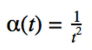
- Does this converge?

- No. Sum of alphas is not infinity
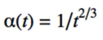
- Does this convergence?

- Nonstationary system은 모델 파라미터 Θ가 시간의 변화에 따라서 상수가 변한다. 광고를 예시를 들면, 광고에 대한 방문자의 선호도는 제품에 대한 소문, 잦은 광고, 노출에 따른 여러가지 이유로 변할 수 있기 때문이다. 이러한 환경의 MAB문제를 Non-stationary 문제라고 한다. 시간에 흐름에 따라 α+β값이 증가함으로 Θ에 대한 추정이 어려워진다.
# From the course: Bayesin Machine Learning in Python: A/B Testing
# https://deeplearningcourses.com/c/bayesian-machine-learning-in-python-ab-testing
# https://www.udemy.com/bayesian-machine-learning-in-python-ab-testing
from __future__ import print_function, division
from builtins import range
# Note: you may need to update your version of future
# sudo pip install -U future


import matplotlib.pyplot as plt
import numpy as np
from bayesian_bandit import Bandit


def run_experiment(p1, p2, p3, N):
  bandits = [Bandit(p1), Bandit(p2), Bandit(p3)]

  data = np.empty(N)

  for i in range(N):
    # thompson sampling
    j = np.argmax([b.sample() for b in bandits])
    x = bandits[j].pull()
    bandits[j].update(x)

    # for the plot
    data[i] = x
  cumulative_average_ctr = np.cumsum(data) / (np.arange(N) + 1)

  # plot moving average ctr
  plt.plot(cumulative_average_ctr)
  plt.plot(np.ones(N)*p1)
  plt.plot(np.ones(N)*p2)
  plt.plot(np.ones(N)*p3)
  plt.ylim((0,1))
  plt.xscale('log')
  plt.show()


run_experiment(0.2, 0.25, 0.3, 100000)
Reference:
Artificial Intelligence Reinforcement Learning
Nonstationary Bandits
- there equations will show up again and again
- what is stationary?
- A stationary process is one whose statistics don’t change over rime(e.g mean)
- weak-sense stationary: mean(1st order statistic) and autocovariance(2nd order statistic) don’t change overtime
- if don’t know covariance let’s check it in here
- strong-sense stationary: entire PDF doesn’t change over time
- SSS -> WSS
- what if our bandits are not stationary? does it make sense to calculate the mean as we have been?
Mean Update Equation
- from earlier:

- some rearranging for convenience:

- Replace 1/t:

- Alpha can be anything(even constant). looks kind of like gradient descent
- One adaptive learning rate used 1/t
Low pass filter
- should look familiar:

- Low-pass filter studied in ML related to RNN(i will post ML too in future)
- Get rid of recurrence(复发):

- Q has exponentially decaying dependence on X
- More emphasis on recent value
Convergence Criteria for Q
- Q will converge if :

- think back to calculus 2(두번쨰)
- constant alpha does not converge
- 1/t does
- if problem is Nonstationary, we don’t want Convergence(融合)(equal weighting of all samples doesn’t make sense) so we will see constant alpha used
- Does this converge?

- No. Sum of alphas is not infinity
- Does this convergence?

- Nonstationary system은 모델 파라미터 Θ가 시간의 변화에 따라서 상수가 변한다. 광고를 예시를 들면, 광고에 대한 방문자의 선호도는 제품에 대한 소문, 잦은 광고, 노출에 따른 여러가지 이유로 변할 수 있기 때문이다. 이러한 환경의 MAB문제를 Non-stationary 문제라고 한다. 시간에 흐름에 따라 α+β값이 증가함으로 Θ에 대한 추정이 어려워진다.
# From the course: Bayesin Machine Learning in Python: A/B Testing
# https://deeplearningcourses.com/c/bayesian-machine-learning-in-python-ab-testing
# https://www.udemy.com/bayesian-machine-learning-in-python-ab-testing
from __future__ import print_function, division
from builtins import range
# Note: you may need to update your version of future
# sudo pip install -U future
import matplotlib.pyplot as plt
import numpy as np
from bayesian_bandit import Bandit
def run_experiment(p1, p2, p3, N):
bandits = [Bandit(p1), Bandit(p2), Bandit(p3)]
data = np.empty(N)
for i in range(N):
# thompson sampling
j = np.argmax([b.sample() for b in bandits])
x = bandits[j].pull()
bandits[j].update(x)
# for the plot
data[i] = x
cumulative_average_ctr = np.cumsum(data) / (np.arange(N) + 1)
# plot moving average ctr
plt.plot(cumulative_average_ctr)
plt.plot(np.ones(N)*p1)
plt.plot(np.ones(N)*p2)
plt.plot(np.ones(N)*p3)
plt.ylim((0,1))
plt.xscale('log')
plt.show()
run_experiment(0.2, 0.25, 0.3, 100000)
Reference:
Artificial Intelligence Reinforcement Learning

Comments