10. Value Function(2) & Bellman Equation
28 Sep 2019 | Reinforcement Learning
Value Function & The Bellman Equation
- The full derivation(起源) can be tough if our probability skills are not yet strong enough
1. Expected Values
- why is this strange to many people?
- Consider a coin toss: Heads = Win, Tails = Lose
- Numerically: H = 1, T = 0
- suppose, P(W) = 60%
- Expected Value is 0.6 x 1 + 0.4 * 0 = 0.6
- The “Expected Value” is a “Value” I can “never expect”
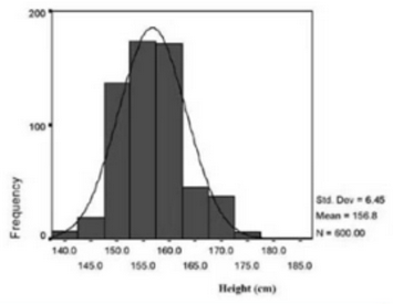
- What’s the point of expected values?
- it tells us the mean/average (E.g. we gather up all the heights of students in the call and calculate the mean- no student may have the mean height, but it’s a useful statistic)
- it doesn’t matter if a coin flip will never give me 0.6, it just an average

- x is state()
2. probability Trees
- our expected reward is the weighted sum of each possible outcome(weighted by the probability at the corresponding branch)
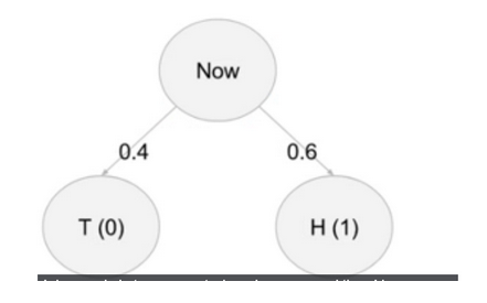
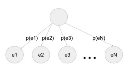
- the same concept extends to any number of possible outcomes
- in general: Expected value = p(e1) x value(e1) + p(e2) x value(e2) + ….
3. Why are averages important?
- A subsection(分部) of a tree is also a tree – recursion(递归)
- After Arriving in this state, what happens next can be considered Random
- Hence, we cannot say: “if i reach this state, i will get X reward”
- we can only say: “if i reach this state, i will get X reward on average”
4. A fundamental concept of The Value Function
- At each state s, i will get a reward R
- overall return G, is the sum of rewards i get
- we want to be able to answer:
- “if i am in state, s what is the sum of reward i will get in the future, on average?”
- we say: V(s) = E(GIs)
- “I” means “givens” - anything to the left is random/ right is not random
- note : this is called a “conditional expectation”
- Value Function is equal to Expected function of Total Return by state

- Every Game we play is just a series of states and rewards
- Let’s pretend everything is deterministic for now, e.g. E(3) = 3
- The value of a state is just the sum of all future rewards(if they are deterministic)
- V($s_1$) = $r_2$ + $r_3$ + $r_4$ + … + $r_N$
- V($s_2$) = $r_3$ + $r_4$ + … + $r_N$
- Key: V($s_1$) = $r_2$ + V($s_2$)
- Discounted Version
- V($s_1$) = $r_2$ + ɣ$r_3$ + ɣ$r_4$ + … + $r_N$
- V($s_2$) = ɣ$r_3$ + ɣ$r_4$ + … + ɣ$r_N$
- Key: V($s_1$) = $r_2$ + ɣV($s_2$)
- (still assuming everything is deterministic)
- In more general terms
- Let’s make s = current state, s’=next state
- Let’s make r = reward(reall means R(s,s’)- the reward i get from going from s to s’)
- V(s) = E[r + ɣV(s’)]
- this is the essence of the bellman equation
- Expansion
- V(s) = E[r + ɣE(r’+ɣV(s’’))]
- V(s) = E[r + ɣE(r’+ɣE(r’‘+…))]
- understanding this “Structure”
- putting more details back in
- s is “given” - we’ve already arrived here
- V(s) = E[r + ɣV(s’) I s]
- Expansion again
- V(s) = state-value function
- Q(s,a) = action-value function
- Q(s,a) = E[GIs,a] = E[r + ɣV(s’) I s,a]
- to understand how Q anv V are related, we need to look at policies(something that tells us what action a to do, given what state we are in)
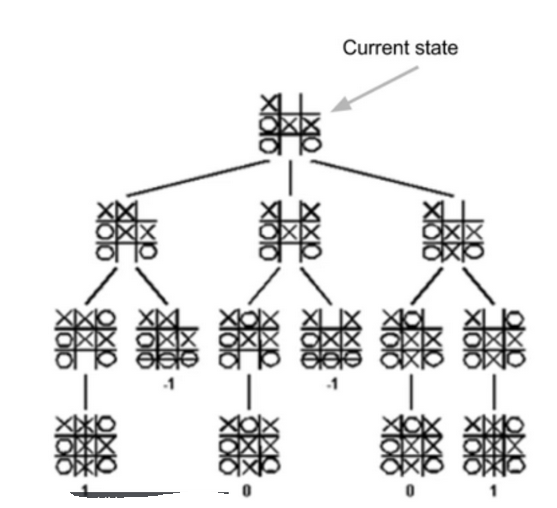
- we know earlier(informally) with tic-tac-Toe
- if any discrepancies(差异) between then and now, consider everything from here onward to be more correct
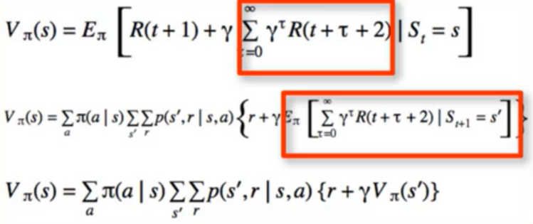
- Value Function is determined by a policy and has state “s” as parameter
- only future rewards
- value of all terminal states is thus 0
- the state value of the terminal state in an episodic problem should always be zero, the value of a state is the expected sum of all future rewards when starting in that state and following a specific policy. for the terminal state, this is zero - there are no more rewards to be end
0

- Recursiveness(递归性)

5. Some Algebra
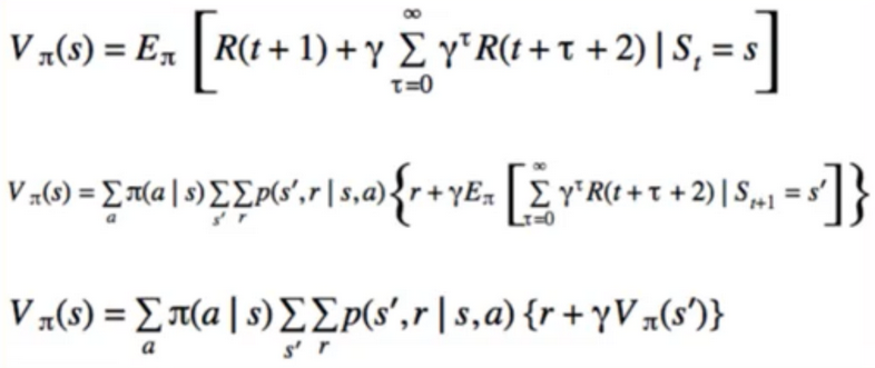
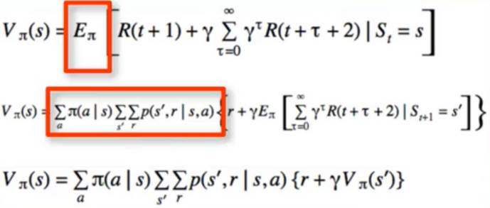
- since the expected value is over π, that means we can express it as a possibility distribute
- π = π(a I s)
- the expected values are linear operators, so we can find each term one at a time

- policy with in return action value in respect to state
- reward and probabilty with return reward in respect to state and action
- in terms of p(s’,r I s,a)

- we can do this for anything
So let’s do it for all of V(s)
- E(E(X)) = E(X)
- we can do this infinity and it won’t change the answer
- E(A+B) = E(A+E(B))
- Therefore if i have one expected value like that, i can insert another expected value in there
- Law of total expectation: E(X)=E(E(X I Y))
- E(E(G(t+1) I ANY)) = E(G(t+1))
- now we know that any condition or expectation could go in that spot
- pick ANY = S(t+1) = s’
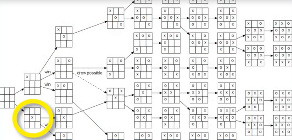
- if i want to know what to do next i just look at what is the reward i get by going there whay is this has to do with how to find an optimal policy.
- Key: No need to enumerate all possible future(which could be infinity long), in order to choose every action
6. Bellman Equation
- Richard bellman
- Pioneered “dynamic programming”
- Bottom-up approach
- DP(dynamic programming) is also one of the solution we’ll study for MDPs

- State-value Fucntion

- Action-value function

- Space Required is quadratic: ISI x IAI
7. Bellman Equation by Example
- Simple models with just a handful of states, easy to solve by hand
- Big Picture perspective: All we want to do is “solve for V(S)”
- ‘Value Function’ represent how good is a state for an agent to be in
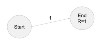
Example 1
- probability of going to end, from start, is 1
- Reward for landing in end is 1
- Discount factor ɣ = 0.9
- Question: what problem are we solving again?
- if we said, “find V(s)”, we are right
- In particular, we want:
- V(START)
- V(End)
- Try it ourselves before moving on
- Remember “Value” is sum of all Future rewards
- Value of Terminal state is always 0
- V(end) = 0
- V(start) = 1
- Note: ɣ only applies to future rewards
- V(start) = R + ɣ(End)
Example 2
- Everything is still deterministic
- Discount factor ɣ = 0.9
- V(End)=0 (terminal state)
- V(Mid)=1 (Takes the role of V(Start) From Example 1)
- V(Start) = R(Start,Mid) + ɣV(Mid) = 0 + 0.9 x 1 = 0.9
Example 3
- V(End) = 0 (unaffected)
- V(Mid) = 1 (Also unaffected, only calculated from future rewards)
- V(Star) = R(Start,Mid) + ɣV(Mid) = -0.1 + 0.9*1 = 0.8
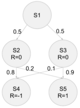
Example 4
- Start at S1
- Discount factor ɣ = 0.9
- Nuance: What do these Probabilities refer to?
- we model games as MDPs - not just coin flips
- as an intelligent agent, our policy tells me what action to do : π(a I s).
- Important : Does not tell me where we go
- p(s’,r I s,a) tells me where i end up
- this example oversimplifies MDPs, but is easier to verbalize(用言语)
- For these examples, we’ll consider the action to be “deciding where to go”
- V(S4) = 0
- V(S2) = 1
- V(S3) = 1 (Same logic as previous examples)
- V(S1) = p(S2 I S1)[R2+ɣV(S2)]+p(S3 I S1)[R3+ɣV(S3)] = 0.5(-0.2 + 0.91)+0.5(-0.3 + 0.91) = 0.65
Example 5
- V(S4), V(S5) =0 (Terminal)
- V(S2) = p(S4 I S2)[R4 + ɣV(S4)] + p(S5 I S2)[R5 + ɣV(S5)] = 0.8-1 + 0.21 = -0.6
- V(S3) = p(S4 I S3)[R4 + ɣV(S4)] + p(S5 I S3)[R5 + ɣV(S5)] = 0.1-1 + 0.91 = 0.8
- V(S1) = p(S2 I S1)[R2 + ɣV(S2)] + p(S3 I S1)[R3 + ɣV(S3)] = 0.5(0.9-0.6) + 0.5(0.9*0.8)= 0.09
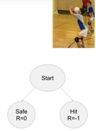
Example 6
- sperate policy randomness from state-arrival randomness
- situation:
- someone throws a ball at me
- our action: either “duck” or “jump”
- next possible states:
- Get hit: R = -1
- Don’t Get hit(safe): R = 0
- the action cannot be “don’t get hit”
- if one could simply choose not to get hit one would never lose
- can aplly to any “real-life” scenario, e.g. starting a company
- π(jump I start) = 0.5
- π(duck I start) = 0.5
p(hit, reward = -1 I jump,start) = 0.8
p(hit, reward = 0 I jump,start) = 0
p(safe, reward = -1 I jump,start) = 0
p(safe, reward = 0 I jump,start) = 0.2
p(hit, reward = -1 I duck,start) = 0.2
p(hit, reward = 0 I duck,start) = 0.4
p(safe, reward = -1 I duck,start) = 0.6
p(safe, reward = 0 I duck,start) = 0.4
- just marginalize over reward since they are really deterministic
p(hit, reward = -1 I jump,start) = 0.8
p(safe, reward = 0 I jump,start) = 0.2

p(hit, reward = 0 I duck,start) = 0.4
p(safe, reward = -1 I duck,start) = 0.6
- as usual, V(safe) and V(hit) = 0
- sanity(明智) check: we should have 4 things to sum over (2 x 2 - think of looping over all possibilities in code)
for brevity(简洁):
Don't show start condition
j = jump, d = duck

V(Start) = π(j)p(safe I j)*0 + π(j)p(hit I j) * (-1) + π(d)p(safe I j)*0 + π(d)p(safe I j)*(-1)
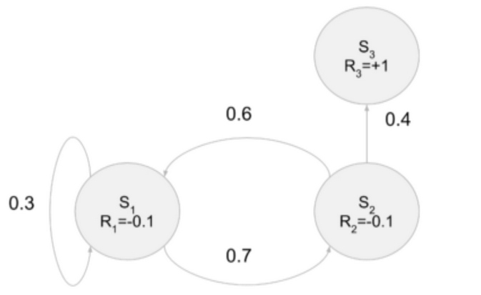
Example 7
- The Previous examples were easy: just work backwards
- Now we have a cycle: no notion of “backwards”
- Back to actions being “go to next state”
- R1 = R2 = -0.1
- Discount Factor ɣ = 0.9
V(s1) = p(s1 I s1)(R1+ɣV(s1)) + p(s2 I s1)(R2 + ɣV(s2))
V(s1) = 0.3(-0.1+0.9V(s1)) + 0.7(-0.1 + 0.9V(s2)) = -0.1 + 0.27V(s1) + 0.63V(s2)
V(s2) = p(s1 I s2)(R1+ɣV(s1)) + p(s3 I s2)(R3 + ɣV(s3))
V(s2) = 0.6(-0.1+0.9V(s1)) + 0.4(1 + 0.9V(s3)) = 0.34 + 0.54V(s1) + 0.36V(s3)
V(s3) = 0
V(s1) = -0.1 + 0.27V(s1) + 0.63V(s2)
V(s2) =0.34 + 0.54V(s1)
V(s3) = 0
- this is linear system (3 equations, 3 unknowns)
0.1   = -0.73V(s1) + 0.63V(s2)
-0.34 = 0.54V(s1) - V(s2) + 0.36V(s3)
0     = V(s3)
- of the form Ax=b
x = np.linalg.solve(A,b)
- V(s1) = 0.293
- V(s2) = 0.498
- V(s3) = 0
7. Bellman Equation Summary
- “Working backwards method”
- “Linear eqaution method”
- big picture:
- Get away from the idea that : “i need to try this on a finance data”, “i need to try this on a biology dataset”, etc.. algorithm doesn’t change, all it sees is a list of numbers
- Rather, we want to know: “ What are scalable algorithms that solve this modelling problem?”
8. Optimal Policies & Optimal Value Functions
- these are interdependent - a key concept in this course - lots of depth to this idea
- we can talk about the relative “goodness” of policies

The Best Policy
- optimal policy is the “best” policy
- the policy for which there is no greater value function

- Optimal Policies are not unique, optimal value functions are :


Relationship Between V and Q
- Implementation advantage:
- to find the best action, we must actually do it to find the best V(s’)
- With Q, we simply need to Look up Q(s,a)

Bellman Optimality Equation
9. Implementing the Optimal Policy
- Key point : Value Function already takes future rewards into account
- Just greedily choose the action that yield the best next-state value V(s’)
- requires look-ahead search
- if we have Q(s,a), no need to look ahead, simply choose argmax
- Q(s,a) thus effectively caches the look-ahead search results
10. step from Value Function to Optimal Policy and Q function
- the value function depends on the policy by which the agent picks actions to perform. so if the agent uses a given policy π to select actions, the corresponding value function is given by :

- among all possible value-functions, there exist an optimal value function that has higher value than other functions for all states

- the optimal policy π is the policy that corresponds to optimal value function.


- In addition to the state value-function, for Convenience RL algorithms introduce another function which is the state-action pair Q-Function. Q is a function of a state-action pair and returns a real value

11. MDP Summary
- Purely Theoretical
- MDPs
- Policies
- Returns-total future reward
- Discounting future rewards with the discount rate, gamma
- state-value function
- action-value function
- bellman equation

- Bellman Optimality Equations
- Next Section:
Reference:
Artificial Intelligence Reinforcement Learning
Value Function & The Bellman Equation
- The full derivation(起源) can be tough if our probability skills are not yet strong enough
1. Expected Values
- why is this strange to many people?
- Consider a coin toss: Heads = Win, Tails = Lose
- Numerically: H = 1, T = 0
- suppose, P(W) = 60%
- Expected Value is 0.6 x 1 + 0.4 * 0 = 0.6
- The “Expected Value” is a “Value” I can “never expect”

- What’s the point of expected values?
- it tells us the mean/average (E.g. we gather up all the heights of students in the call and calculate the mean- no student may have the mean height, but it’s a useful statistic)
- it doesn’t matter if a coin flip will never give me 0.6, it just an average

- x is state()
2. probability Trees
- our expected reward is the weighted sum of each possible outcome(weighted by the probability at the corresponding branch)

- the same concept extends to any number of possible outcomes
- in general: Expected value = p(e1) x value(e1) + p(e2) x value(e2) + ….

3. Why are averages important?
- A subsection(分部) of a tree is also a tree – recursion(递归)
- After Arriving in this state, what happens next can be considered Random
- Hence, we cannot say: “if i reach this state, i will get X reward”
- we can only say: “if i reach this state, i will get X reward on average”
4. A fundamental concept of The Value Function
- At each state s, i will get a reward R
- overall return G, is the sum of rewards i get
- we want to be able to answer:
- “if i am in state, s what is the sum of reward i will get in the future, on average?”
- we say: V(s) = E(GIs)
- “I” means “givens” - anything to the left is random/ right is not random
- note : this is called a “conditional expectation”
- Value Function is equal to Expected function of Total Return by state

- Every Game we play is just a series of states and rewards
- Let’s pretend everything is deterministic for now, e.g. E(3) = 3
- The value of a state is just the sum of all future rewards(if they are deterministic)
- V($s_1$) = $r_2$ + $r_3$ + $r_4$ + … + $r_N$
- V($s_2$) = $r_3$ + $r_4$ + … + $r_N$
- Key: V($s_1$) = $r_2$ + V($s_2$)
- Discounted Version
- V($s_1$) = $r_2$ + ɣ$r_3$ + ɣ$r_4$ + … + $r_N$
- V($s_2$) = ɣ$r_3$ + ɣ$r_4$ + … + ɣ$r_N$
- Key: V($s_1$) = $r_2$ + ɣV($s_2$)
- (still assuming everything is deterministic)
- In more general terms
- Let’s make s = current state, s’=next state
- Let’s make r = reward(reall means R(s,s’)- the reward i get from going from s to s’)
- V(s) = E[r + ɣV(s’)]
- this is the essence of the bellman equation
- Expansion
- V(s) = E[r + ɣE(r’+ɣV(s’’))]
- V(s) = E[r + ɣE(r’+ɣE(r’‘+…))]
- understanding this “Structure”
- putting more details back in
- s is “given” - we’ve already arrived here
- V(s) = E[r + ɣV(s’) I s]
- Expansion again
- V(s) = state-value function
- Q(s,a) = action-value function
- Q(s,a) = E[GIs,a] = E[r + ɣV(s’) I s,a]
- to understand how Q anv V are related, we need to look at policies(something that tells us what action a to do, given what state we are in)
- we know earlier(informally) with tic-tac-Toe
- if any discrepancies(差异) between then and now, consider everything from here onward to be more correct
- Value Function is determined by a policy and has state “s” as parameter
- only future rewards
- value of all terminal states is thus 0
- the state value of the terminal state in an episodic problem should always be zero, the value of a state is the expected sum of all future rewards when starting in that state and following a specific policy. for the terminal state, this is zero - there are no more rewards to be end
0

- Recursiveness(递归性)

5. Some Algebra
- since the expected value is over π, that means we can express it as a possibility distribute
- π = π(a I s)
- the expected values are linear operators, so we can find each term one at a time

- policy with in return action value in respect to state
- reward and probabilty with return reward in respect to state and action
- in terms of p(s’,r I s,a)

- we can do this for anything
So let’s do it for all of V(s)
- E(E(X)) = E(X)
- we can do this infinity and it won’t change the answer
- E(A+B) = E(A+E(B))
- Therefore if i have one expected value like that, i can insert another expected value in there
- Law of total expectation: E(X)=E(E(X I Y))
- E(E(G(t+1) I ANY)) = E(G(t+1))
- now we know that any condition or expectation could go in that spot
- pick ANY = S(t+1) = s’

- if i want to know what to do next i just look at what is the reward i get by going there whay is this has to do with how to find an optimal policy.
- Key: No need to enumerate all possible future(which could be infinity long), in order to choose every action
6. Bellman Equation
- Richard bellman
- Pioneered “dynamic programming”
- Bottom-up approach
- DP(dynamic programming) is also one of the solution we’ll study for MDPs

- State-value Fucntion

- Action-value function

- Space Required is quadratic: ISI x IAI
7. Bellman Equation by Example
- Simple models with just a handful of states, easy to solve by hand
- Big Picture perspective: All we want to do is “solve for V(S)”
- ‘Value Function’ represent how good is a state for an agent to be in
Example 1
- probability of going to end, from start, is 1
- Reward for landing in end is 1
- Discount factor ɣ = 0.9
- Question: what problem are we solving again?
- if we said, “find V(s)”, we are right
- In particular, we want:
- V(START)
- V(End)
- Try it ourselves before moving on
- Remember “Value” is sum of all Future rewards
- Value of Terminal state is always 0
- V(end) = 0
- V(start) = 1
- Note: ɣ only applies to future rewards
- V(start) = R + ɣ(End)
Example 2
- Everything is still deterministic
- Discount factor ɣ = 0.9
- V(End)=0 (terminal state)
- V(Mid)=1 (Takes the role of V(Start) From Example 1)
- V(Start) = R(Start,Mid) + ɣV(Mid) = 0 + 0.9 x 1 = 0.9
Example 3
- V(End) = 0 (unaffected)
- V(Mid) = 1 (Also unaffected, only calculated from future rewards)
- V(Star) = R(Start,Mid) + ɣV(Mid) = -0.1 + 0.9*1 = 0.8
Example 4
- Start at S1
- Discount factor ɣ = 0.9
- Nuance: What do these Probabilities refer to?
- we model games as MDPs - not just coin flips
- as an intelligent agent, our policy tells me what action to do : π(a I s).
- Important : Does not tell me where we go
- p(s’,r I s,a) tells me where i end up
- this example oversimplifies MDPs, but is easier to verbalize(用言语)
- For these examples, we’ll consider the action to be “deciding where to go”
- V(S4) = 0
- V(S2) = 1
- V(S3) = 1 (Same logic as previous examples)
- V(S1) = p(S2 I S1)[R2+ɣV(S2)]+p(S3 I S1)[R3+ɣV(S3)] = 0.5(-0.2 + 0.91)+0.5(-0.3 + 0.91) = 0.65
Example 5
- V(S4), V(S5) =0 (Terminal)
- V(S2) = p(S4 I S2)[R4 + ɣV(S4)] + p(S5 I S2)[R5 + ɣV(S5)] = 0.8-1 + 0.21 = -0.6
- V(S3) = p(S4 I S3)[R4 + ɣV(S4)] + p(S5 I S3)[R5 + ɣV(S5)] = 0.1-1 + 0.91 = 0.8
- V(S1) = p(S2 I S1)[R2 + ɣV(S2)] + p(S3 I S1)[R3 + ɣV(S3)] = 0.5(0.9-0.6) + 0.5(0.9*0.8)= 0.09
Example 6
- sperate policy randomness from state-arrival randomness
- situation:
- someone throws a ball at me
- our action: either “duck” or “jump”
- next possible states:
- Get hit: R = -1
- Don’t Get hit(safe): R = 0
- the action cannot be “don’t get hit”
- if one could simply choose not to get hit one would never lose
- can aplly to any “real-life” scenario, e.g. starting a company
- π(jump I start) = 0.5
- π(duck I start) = 0.5
p(hit, reward = -1 I jump,start) = 0.8
p(hit, reward = 0 I jump,start) = 0
p(safe, reward = -1 I jump,start) = 0
p(safe, reward = 0 I jump,start) = 0.2
p(hit, reward = -1 I duck,start) = 0.2
p(hit, reward = 0 I duck,start) = 0.4
p(safe, reward = -1 I duck,start) = 0.6
p(safe, reward = 0 I duck,start) = 0.4
- just marginalize over reward since they are really deterministic
p(hit, reward = -1 I jump,start) = 0.8
p(safe, reward = 0 I jump,start) = 0.2
p(hit, reward = 0 I duck,start) = 0.4
p(safe, reward = -1 I duck,start) = 0.6
- as usual, V(safe) and V(hit) = 0
- sanity(明智) check: we should have 4 things to sum over (2 x 2 - think of looping over all possibilities in code)
for brevity(简洁):
Don't show start condition
j = jump, d = duck
V(Start) = π(j)p(safe I j)*0 + π(j)p(hit I j) * (-1) + π(d)p(safe I j)*0 + π(d)p(safe I j)*(-1)
Example 7
- The Previous examples were easy: just work backwards
- Now we have a cycle: no notion of “backwards”
- Back to actions being “go to next state”
- R1 = R2 = -0.1
- Discount Factor ɣ = 0.9
V(s1) = p(s1 I s1)(R1+ɣV(s1)) + p(s2 I s1)(R2 + ɣV(s2))
V(s1) = 0.3(-0.1+0.9V(s1)) + 0.7(-0.1 + 0.9V(s2)) = -0.1 + 0.27V(s1) + 0.63V(s2)
V(s2) = p(s1 I s2)(R1+ɣV(s1)) + p(s3 I s2)(R3 + ɣV(s3))
V(s2) = 0.6(-0.1+0.9V(s1)) + 0.4(1 + 0.9V(s3)) = 0.34 + 0.54V(s1) + 0.36V(s3)
V(s3) = 0
V(s1) = -0.1 + 0.27V(s1) + 0.63V(s2)
V(s2) =0.34 + 0.54V(s1)
V(s3) = 0
- this is linear system (3 equations, 3 unknowns)
0.1 = -0.73V(s1) + 0.63V(s2)
-0.34 = 0.54V(s1) - V(s2) + 0.36V(s3)
0 = V(s3)
- of the form Ax=b x = np.linalg.solve(A,b)
- V(s1) = 0.293
- V(s2) = 0.498
- V(s3) = 0
7. Bellman Equation Summary
- “Working backwards method”
- “Linear eqaution method”
- big picture:
- Get away from the idea that : “i need to try this on a finance data”, “i need to try this on a biology dataset”, etc.. algorithm doesn’t change, all it sees is a list of numbers
- Rather, we want to know: “ What are scalable algorithms that solve this modelling problem?”
8. Optimal Policies & Optimal Value Functions
- these are interdependent - a key concept in this course - lots of depth to this idea
- we can talk about the relative “goodness” of policies

The Best Policy
- optimal policy is the “best” policy
- the policy for which there is no greater value function

- Optimal Policies are not unique, optimal value functions are :


Relationship Between V and Q
- Implementation advantage:
- to find the best action, we must actually do it to find the best V(s’)
- With Q, we simply need to Look up Q(s,a)

Bellman Optimality Equation
9. Implementing the Optimal Policy
- Key point : Value Function already takes future rewards into account
- Just greedily choose the action that yield the best next-state value V(s’)
- requires look-ahead search
- if we have Q(s,a), no need to look ahead, simply choose argmax
- Q(s,a) thus effectively caches the look-ahead search results
10. step from Value Function to Optimal Policy and Q function
- the value function depends on the policy by which the agent picks actions to perform. so if the agent uses a given policy π to select actions, the corresponding value function is given by :

- among all possible value-functions, there exist an optimal value function that has higher value than other functions for all states

- the optimal policy π is the policy that corresponds to optimal value function.


- In addition to the state value-function, for Convenience RL algorithms introduce another function which is the state-action pair Q-Function. Q is a function of a state-action pair and returns a real value

11. MDP Summary
- Purely Theoretical
- MDPs
- Policies
- Returns-total future reward
- Discounting future rewards with the discount rate, gamma
- state-value function
- action-value function
- bellman equation

- Bellman Optimality Equations
- Next Section:
Reference:
Artificial Intelligence Reinforcement Learning








Comments