13. TD Temporal Difference Learning
29 Sep 2019 | Reinforcement Learning
Temporal Difference (TD) Learning
- this section is a 3rd technique for solving MDPs
- TD = Temporal Difference(TD) Learning
- Combines ideas from DP and MC
- Disadvantage of DP: requires full model of environment, never learns from experience
- MC and TD learn from experience
- MC can only update after completing episode, but DP uses Bootstrapping(Making an initial estimate)
- We will see that TD also uses Bootstrapping and is fully online, can update value during an episode
1. TD Learning
- Same approach as before
- First Predict Problem
- them control problem
- 2 control methods:
- SARSA
- Q-Learning
- Model-Free Reinforcement Learning
- TD methods learn directly from episode of experience.
- no Knowledge of MDP Transition / rewards
- TD learns from incomplete episodes by Bootstrapping
- TD updates a guess towards a guess
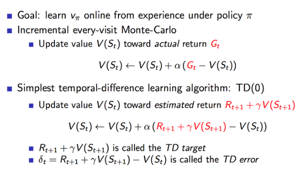
- MC와 다른점은, MC는 실제 에피소드가 끝나고 받게 되는 보상을 사용하여 Value Function을 업데이트 하였다
- TD에서는 실제 보상과 다음 step에 대한 미래추정가치를 사용해서 학습한다.
- 이때 사용하는 보상과 Value Function의 합을 TD Target
-그리고 TD Target 과 실제 V(S)와의 차이를 TD error라고 표현한다.
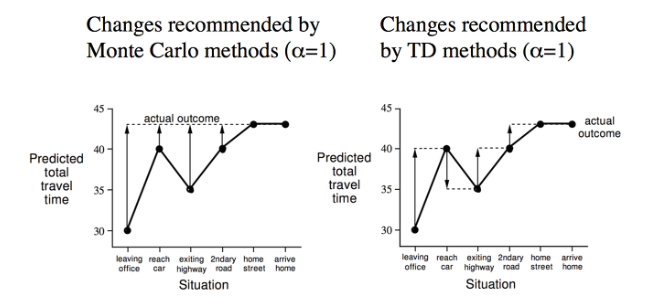
- MC에서의 Value function이 업데이트 되는 과정이 왼쪽(에피소드가 전체적으로 끝나서 그의 보상을 나누어 단계별로 업데이트)
- TD는 각 단계별로 업데이트가 되는 과정으로 오른쪽 그림
- TD의 장점은 에피소드 중간에서도 학습을 하게 된다는 것이다.
- MC에서는 에피소드가 끝날때까지 기다렸다가 업데이트가 발생하고 학습하기 떄문이다.
- TD는 종료 없는 연속적인 에피소드에서도 학습할 수 있다.
- Return $G_t$ = R(t+1)+ɣR(t+2)+…+ɣ^(t-1)$R_T) is unbiased estimate of $v_π$($S_t$)
- True TD Target R(t+1)+ɣV(S(t+1)) is biased estimate of $v_π$($S_t$)
- TD Target is much lower variance than the return:
- return depends on many random actions, transitions, rewards
- TD Target depends on one random action, transition, reward
- V policy가 실제 G에 대해서 unbias라 할때는 TD Target도 V policy를 추종하기 unbias이다. 하지만 TD Target에 V policy를 추정하는 V(St+1)를 사용하기에 실제값이 아니라 실제값을 추정하는 값임으로 bias가 발생한다. 그리고 TD Target은 단지 하나의 step에서만 계산하기에 noise가 작게 되므로 상대적으로 variance가 낮게 나타난다.
- MC has high variance, zero bias
- good convergence properties
- even with function approximation
- not very sensitive to initial value
- very simple to understand and use
- TD has low variance, some bias
- Usually more efficient than MC
- TD(0) converges to $v_π$(s)
- but not always with function approximation
- More sensitive to initial value
- Compare on variance between MC and TD
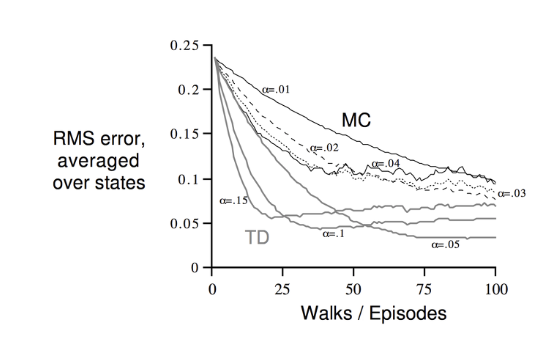
- Bootstrapping이 더 학습하는데 효율적이다.
- MC and TD converge : V(s) -> $v_π$(s) as experience -> ∞ (에피소드는 무한 반복하게 되면 결국 수렴하게 되어있다.)
- but what about batch solution for finite experience
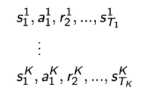
- e.g repeatedly sample episode k ∈ [1,K]
- Apply MC or TD(0) to episode k
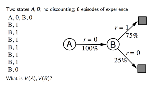
- For example, first episode A got reward “0” and B got reward “0”
- from Second Episode B got reward “1” to seven episode. and B got 0 at the last episode.
- then A will go B within 100 % and then reward will be “0”
- in the MC methods, A will get reward “0” because the episode pass Through A is one that final reward is zero
6- in the TD methods, running another episode because of B value update to “6” then A value also going to be updated
- MC converges to solution with minimum mean-square
- TD(0) converges to solution of max likelihood Markov Model
- TD(0)방식은 max likelihood Markv 방식을 사용하여 수렴하는 알고리즘이다. MDP 기반으로 실제적인 값을 찾아가게 되기 때문에 V(A)의 값이 6/8 평균가치가 계산되어 0.75값으로 업데이트가 된다.
- TD exploits Markov property
- Usually more efficient in Markov environment
- MC does not exploit Markov property
- Usually more effective in Non-Markov environment
- MC 알고르짐
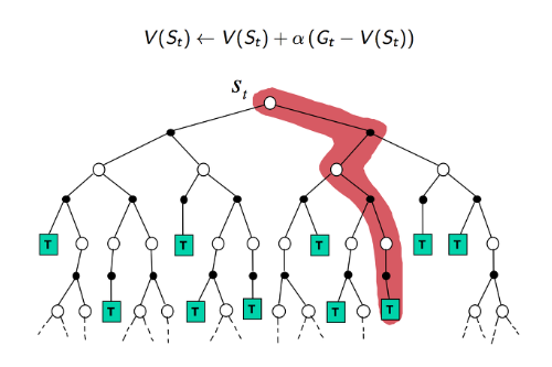
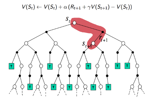
- Bootstrapping을 사용하여 states에 대한 value들을 추정하여 사용하는 방법 TD
- DP 방식
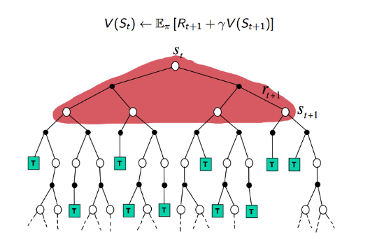
- DP 방식에서는 모델을 통해서 이미 MDP를 알고 있고 이에 대한 value 와 reward를 통해 학습을 하기 때문에 위에와 같이 나옵니다.
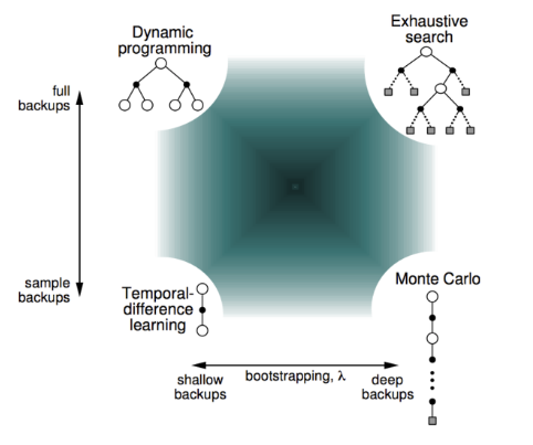
- Bootstrapping: update involves an estimate
- MC does not bootstrap
- DP bootstraps
- TD bootstrap
- Sampling update samples an expectation
- MC samples
- DP does not sample
- TD samples
- DP와 TP에서 사용하는 Bootstrapping은 추정 값을 기반으로 하여 업데이트
- MC에서 사용하는 샘플링은 expectation을 샘플하여 업데이트 한다.
- TD도 샘플링을 한지만 DP처럼 full backup을 하지 않는다.
2. TD(0) Prediction
- Apply TD to prediction problem
- algorithm is called TD(0)
- there is also TD(1) and TD(λ)
- it is related to Q-Learning and approximation methods
MC
- Recall: one Disadvantage of MC is we need to wait until the episode is finished then we calculate return
- also recall: Multiple ways of calculating averages
- General “average-finding” equation
- Does not require us to store all returns
- Constant alpha is moving average/exponential decay

Value function
TD(0)
- can we just combine these(MC & Value Function)
- instead of sampling the return, use the recursive definition

- this is TD(0)
- why this is fully online? we can update V(s) as soon as we know s’
sources of randomness
- In Mc, randomness arises when an episode can play out in different ways(due to stochastic policy, or stochastic state transitions)
- in TD(0), we have another source of randomness
- G is an exact sample in MC
- r + ɣV(s’) is itself an estimate of G
- we are estimating from other estimates(bootstrapping)
Summary
- TD(0) is advantageous in comparison to MC/DP
- Unlike DP, we don’t require a model of the environment, and only update V for states we visit
- unlike MC, we don’t need to wait for an episode to finish
- advantageous for very long episodes
- also applicable to continuous(non-episodic)tasks
3. TD Learning for Control
- Apply TD(0) to Control
- we can probably guess what we’re going to do by now
- use Generalized policy iteration, alternate between TD(0) for prediction, policy improvement using greedy action selection
- Use Value iteration method: Update Q in-place, improve policy after every change
- skip the part where we do full policy evaluation
4. SARSA
- Recall from MC: we want to use Q because it’s indexed by a, V is only indexed by s
- Q has the same recursive form
- Same limitation as MC: need lots of samples in order to converge
- require the 5-tuuple:(s,a,r,s’,a’)
- Hence the name

- TD방식과 다른점은 Value function을 쓰지 않고 Q Fucntion을 쓴다.
- Like MC, still requires us to know Q(s,a) for all a, in order to choose argmax
- problem: if we follow a deterministic policy, we would only fill in 1/IAI values on each episode
- Leave most of Q untouched
- Remedy(处理方法): Exploring starts or policy that includes exploration
- use epsilon-greedy
Pseudocode
Q(s,a) = arbitrary, Q(terminal,a) = 0
for t=1..N
  s = start_state, a = epsilon_greedy_from(Q(s))
  while not game over:
    s', r = do_action(a)
    a' = episode_greedy_from(Q(s'))
    Q(s,a) = Q(s,a) + alpha + [r + gamma*Q(s',a')-Q(s,a)]
    s = s', a = q'
- Interesting fact : convergence proof has never been published
- has been stated informally that it will converge of policy converges to greedy
- we can achieve this by seeing ε = 1/t
- Or ε = c/t or ε= c/$t^a$
- Hyperparameters
Learning Rate
- Recall that learning rate can also decay
- problem:
- if we set α = 1/t
- at every iteration, only one (s,a) pair will be updated for Q(s,a)
- Learning rate will decay even for values we have never updated
- Could we just only decrease α after every episode?
- No
- Many elements of Q(s,a) are not updated during an episode
- we take inspiration from deep learning: AdaGrad and RMSprop(adaptive learning rates)
- Effective Learning rate Decays more when previous gradient has been larger
- in other words: the more it has changed in the past, the less it will change in the future
- our version is simpler: keep a count of every(s,a) pair seen:
- α(s,a) = $α_0$ / count(s,a)
- Equivalently
- α(s,a) = $α_0$ / (k+m*count(s,a))
5. Q-Learning
- Main Theme: Generalize policy iteration
- Policy evaluation
- Policy Improvement(greedy wrt(with regard to) current value)
- what we’ve been studying: on-policy methods
- we always follow the current best policy
- Q-Learning is an off-policy methds
- do any random action, and still find Q*
- Looks similar SARSA

- instead of choosing a’ based on argmax of Q, we update Q(s,a) directly with max over Q(s’,a’)
- isn’t that the same, since a’=argmax[a’]{Q(s’,a’)}?

- we don’t need to actually do action a’ as the next move
- therefore, we use Q(s’,a’) in the update for Q(s,a), even if we don’t do a’ next
- Doesn’t matter what policy we follow
- Reality: Random actions -> suboptimal(then use greed) -> takes longer for episode to finish
- takeaway: doesn’t matter what policy we use
- Under What circumstance is Q-learning == SARSA?
- if policy used for Q-learning is greedy
- then we’ll be doing Sarsa, but we also be doing Q-Learning
6.Summary
- TD combines aspects of MC and DP
- MC: Learn From experience / play the game
- Generalized idea of taking sample mean of returns
- Multi-armed bandit
- MC is not fully online
- DP: bootstrapping, recursive from of value function
- TD(0) = MC + DP (combines)
- Instead of taking sample mean of returns, we take sample mean of estimated returns, based on r and V(s’)
TD Summary
- Control
- On-policy: SARSA
- Off-policy : Q-Learning
TD Disadvantage
- Need Q(s,a)
- state space can easily become infeasible to enumerate
- need to enumerate every action for every state
- Q may not even fit into memory
- Measuring Q(s,a) for all s and a is called the tabular(表格式的) method
- Next, we will learn about function approximated methods which allow us to compress the amount of space needed to represent Q
Reference:
Artificial Intelligence Reinforcement Learning
Temporal Difference (TD) Learning
- this section is a 3rd technique for solving MDPs
- TD = Temporal Difference(TD) Learning
- Combines ideas from DP and MC
- Disadvantage of DP: requires full model of environment, never learns from experience
- MC and TD learn from experience
- MC can only update after completing episode, but DP uses Bootstrapping(Making an initial estimate)
- We will see that TD also uses Bootstrapping and is fully online, can update value during an episode
1. TD Learning
- Same approach as before
- First Predict Problem
- them control problem
- 2 control methods:
- SARSA
- Q-Learning
- Model-Free Reinforcement Learning
- TD methods learn directly from episode of experience.
- no Knowledge of MDP Transition / rewards
- TD learns from incomplete episodes by Bootstrapping
- TD updates a guess towards a guess

- MC와 다른점은, MC는 실제 에피소드가 끝나고 받게 되는 보상을 사용하여 Value Function을 업데이트 하였다
- TD에서는 실제 보상과 다음 step에 대한 미래추정가치를 사용해서 학습한다.
- 이때 사용하는 보상과 Value Function의 합을 TD Target
-그리고 TD Target 과 실제 V(S)와의 차이를 TD error라고 표현한다.

- MC에서의 Value function이 업데이트 되는 과정이 왼쪽(에피소드가 전체적으로 끝나서 그의 보상을 나누어 단계별로 업데이트)
- TD는 각 단계별로 업데이트가 되는 과정으로 오른쪽 그림
- TD의 장점은 에피소드 중간에서도 학습을 하게 된다는 것이다.
- MC에서는 에피소드가 끝날때까지 기다렸다가 업데이트가 발생하고 학습하기 떄문이다.
- TD는 종료 없는 연속적인 에피소드에서도 학습할 수 있다.
- Return $G_t$ = R(t+1)+ɣR(t+2)+…+ɣ^(t-1)$R_T) is unbiased estimate of $v_π$($S_t$)
- True TD Target R(t+1)+ɣV(S(t+1)) is biased estimate of $v_π$($S_t$)
- TD Target is much lower variance than the return:
- return depends on many random actions, transitions, rewards
- TD Target depends on one random action, transition, reward
- V policy가 실제 G에 대해서 unbias라 할때는 TD Target도 V policy를 추종하기 unbias이다. 하지만 TD Target에 V policy를 추정하는 V(St+1)를 사용하기에 실제값이 아니라 실제값을 추정하는 값임으로 bias가 발생한다. 그리고 TD Target은 단지 하나의 step에서만 계산하기에 noise가 작게 되므로 상대적으로 variance가 낮게 나타난다.
- MC has high variance, zero bias
- good convergence properties
- even with function approximation
- not very sensitive to initial value
- very simple to understand and use
- TD has low variance, some bias
- Usually more efficient than MC
- TD(0) converges to $v_π$(s)
- but not always with function approximation
- More sensitive to initial value
- Compare on variance between MC and TD

- Bootstrapping이 더 학습하는데 효율적이다.
- MC and TD converge : V(s) -> $v_π$(s) as experience -> ∞ (에피소드는 무한 반복하게 되면 결국 수렴하게 되어있다.)
- but what about batch solution for finite experience

- e.g repeatedly sample episode k ∈ [1,K]
- Apply MC or TD(0) to episode k

- For example, first episode A got reward “0” and B got reward “0”
- from Second Episode B got reward “1” to seven episode. and B got 0 at the last episode.
- then A will go B within 100 % and then reward will be “0”
- in the MC methods, A will get reward “0” because the episode pass Through A is one that final reward is zero 6- in the TD methods, running another episode because of B value update to “6” then A value also going to be updated
- MC converges to solution with minimum mean-square
- TD(0) converges to solution of max likelihood Markov Model
- TD(0)방식은 max likelihood Markv 방식을 사용하여 수렴하는 알고리즘이다. MDP 기반으로 실제적인 값을 찾아가게 되기 때문에 V(A)의 값이 6/8 평균가치가 계산되어 0.75값으로 업데이트가 된다.
- TD exploits Markov property
- Usually more efficient in Markov environment
- MC does not exploit Markov property
- Usually more effective in Non-Markov environment
- MC 알고르짐

- Bootstrapping을 사용하여 states에 대한 value들을 추정하여 사용하는 방법 TD

- DP 방식

- DP 방식에서는 모델을 통해서 이미 MDP를 알고 있고 이에 대한 value 와 reward를 통해 학습을 하기 때문에 위에와 같이 나옵니다.
- Bootstrapping: update involves an estimate
- MC does not bootstrap
- DP bootstraps
- TD bootstrap
- Sampling update samples an expectation
- MC samples
- DP does not sample
- TD samples
- DP와 TP에서 사용하는 Bootstrapping은 추정 값을 기반으로 하여 업데이트
- MC에서 사용하는 샘플링은 expectation을 샘플하여 업데이트 한다.
- TD도 샘플링을 한지만 DP처럼 full backup을 하지 않는다.

2. TD(0) Prediction
- Apply TD to prediction problem
- algorithm is called TD(0)
- there is also TD(1) and TD(λ)
- it is related to Q-Learning and approximation methods
MC
- Recall: one Disadvantage of MC is we need to wait until the episode is finished then we calculate return
- also recall: Multiple ways of calculating averages
- General “average-finding” equation
- Does not require us to store all returns
- Constant alpha is moving average/exponential decay

Value function
TD(0)
- can we just combine these(MC & Value Function)
- instead of sampling the return, use the recursive definition

- this is TD(0)
- why this is fully online? we can update V(s) as soon as we know s’
sources of randomness
- In Mc, randomness arises when an episode can play out in different ways(due to stochastic policy, or stochastic state transitions)
- in TD(0), we have another source of randomness
- G is an exact sample in MC
- r + ɣV(s’) is itself an estimate of G
- we are estimating from other estimates(bootstrapping)
Summary
- TD(0) is advantageous in comparison to MC/DP
- Unlike DP, we don’t require a model of the environment, and only update V for states we visit
- unlike MC, we don’t need to wait for an episode to finish
- advantageous for very long episodes
- also applicable to continuous(non-episodic)tasks
3. TD Learning for Control
- Apply TD(0) to Control
- we can probably guess what we’re going to do by now
- use Generalized policy iteration, alternate between TD(0) for prediction, policy improvement using greedy action selection
- Use Value iteration method: Update Q in-place, improve policy after every change
- skip the part where we do full policy evaluation
4. SARSA
- Recall from MC: we want to use Q because it’s indexed by a, V is only indexed by s
- Q has the same recursive form
- Same limitation as MC: need lots of samples in order to converge
- require the 5-tuuple:(s,a,r,s’,a’)
- Hence the name

- TD방식과 다른점은 Value function을 쓰지 않고 Q Fucntion을 쓴다.
- Like MC, still requires us to know Q(s,a) for all a, in order to choose argmax
- problem: if we follow a deterministic policy, we would only fill in 1/IAI values on each episode
- Leave most of Q untouched
- Remedy(处理方法): Exploring starts or policy that includes exploration
- use epsilon-greedy
Pseudocode
Q(s,a) = arbitrary, Q(terminal,a) = 0
for t=1..N
s = start_state, a = epsilon_greedy_from(Q(s))
while not game over:
s', r = do_action(a)
a' = episode_greedy_from(Q(s'))
Q(s,a) = Q(s,a) + alpha + [r + gamma*Q(s',a')-Q(s,a)]
s = s', a = q'
- Interesting fact : convergence proof has never been published
- has been stated informally that it will converge of policy converges to greedy
- we can achieve this by seeing ε = 1/t
- Or ε = c/t or ε= c/$t^a$
- Hyperparameters
Learning Rate
- Recall that learning rate can also decay
- problem:
- if we set α = 1/t
- at every iteration, only one (s,a) pair will be updated for Q(s,a)
- Learning rate will decay even for values we have never updated
- Could we just only decrease α after every episode?
- No
- Many elements of Q(s,a) are not updated during an episode
- we take inspiration from deep learning: AdaGrad and RMSprop(adaptive learning rates)
- Effective Learning rate Decays more when previous gradient has been larger
- in other words: the more it has changed in the past, the less it will change in the future
- our version is simpler: keep a count of every(s,a) pair seen:
- α(s,a) = $α_0$ / count(s,a)
- Equivalently
- α(s,a) = $α_0$ / (k+m*count(s,a))
5. Q-Learning
- Main Theme: Generalize policy iteration
- Policy evaluation
- Policy Improvement(greedy wrt(with regard to) current value)
- what we’ve been studying: on-policy methods
- we always follow the current best policy
- Q-Learning is an off-policy methds
- do any random action, and still find Q*
- Looks similar SARSA

- instead of choosing a’ based on argmax of Q, we update Q(s,a) directly with max over Q(s’,a’)
- isn’t that the same, since a’=argmax[a’]{Q(s’,a’)}?

- we don’t need to actually do action a’ as the next move
- therefore, we use Q(s’,a’) in the update for Q(s,a), even if we don’t do a’ next
- Doesn’t matter what policy we follow
- Reality: Random actions -> suboptimal(then use greed) -> takes longer for episode to finish
- takeaway: doesn’t matter what policy we use
- Under What circumstance is Q-learning == SARSA?
- if policy used for Q-learning is greedy
- then we’ll be doing Sarsa, but we also be doing Q-Learning
6.Summary
- TD combines aspects of MC and DP
- MC: Learn From experience / play the game
- Generalized idea of taking sample mean of returns
- Multi-armed bandit
- MC is not fully online
- DP: bootstrapping, recursive from of value function
- TD(0) = MC + DP (combines)
- Instead of taking sample mean of returns, we take sample mean of estimated returns, based on r and V(s’)
TD Summary
- Control
- On-policy: SARSA
- Off-policy : Q-Learning
TD Disadvantage
- Need Q(s,a)
- state space can easily become infeasible to enumerate
- need to enumerate every action for every state
- Q may not even fit into memory
- Measuring Q(s,a) for all s and a is called the tabular(表格式的) method
- Next, we will learn about function approximated methods which allow us to compress the amount of space needed to represent Q
Reference:
Artificial Intelligence Reinforcement Learning


Comments