20. RBF Neural Networks
04 Oct 2019 | Reinforcement Learning
RBF Networks
- RBF = Radial Basis Function
- Useful in RL
- 2 perspectives
- Linear model with feature extraction, where the feature extraction is RBF kernel
- 1-hidden layer neural network, with RBF kernel as activation function
- when we first learned about neural networks, we learned these in reverse order
- we first learned that a neural network is a nonlinear function approximator
- later, we saw that hidden units happen to learn features
RBF Basis Function
- is a non-normalized Gaussian

- x = input vector
- c = center / exemplar(模范) vector
- Only Repends on distance between x and c, not direction, hence the term radial
- Max is 1, when x == c, approaches 0 as x goes further away from c
How do we choose c?
- how many c’s should we choose?
- number of center / exemplar == number of hidden units in the RBF Network
- Each unit will have a different center
- A few different ways to choose them
Support Vecotr Machines
- SVMs also use RBF Kernels
- # of exemplars == # of training points
- in fact, with SVMs the exemplars are the training points
- this is why SVMs have fallen out of favour
- Training becomes O(N^2), prediction is O(N), N = # Training samples
- important piece of deep learning history
- SVMs were once though to be superior
Another Methods
- Just sample a few points from the state space
- can then choose the # of exemplars
- env.observation_sapce.sample()
- how many exemplars we choose is like how many hidden units in a neural network - it’s hyperparameter that must be tuned
Implementation
- we’ll make use of sci-kit learn
- our own difect from-definition implementation would be unnecessarily slow
- RBFsampler uses a Monte Carlo algorithms(MC)
from sklearn.kernel_approximation import RBFsampler
- Standard Interface
sampler = RBFSampler()
sampler.fit(radw_data)
features = sampler.transform(raw_data)
The rest we have done before
- now that we know how to transform the raw state, the rest we should be familiar with: Q-learning, linear function approximation with gradient descent
- Unlike a feedforward neural network, the features won’t change as we learn
- exemplar we choose at the beginning will remain forever
- May seem restrictive, but works better than feedforward NN
Old Perspective vs New Perspective
- we used linear functions with polynomial features before
- now we use RBF Kernel for features
- the other Perspective: 1-hidden layer neural network
- remember that in general, this is a nonlinear transformation -> linear model at the final layer
- Recall: dot product is a cosine distance: $a^T$b = IaI IbI cos(angle(a,b))


Implementation Details
- Scale parameter(aka. Variance)
- We don’t know what’s good
- Perhaps multiple are good
- sci-kit learn has facilities that allow us to use multiple RBF samplers simultaneously
from sklearn.pipeline import FeatureUnion
- Can concatenate(连在一起的) any features, not just those from RBFSampler
- Standardize our data too:
from sklearn.preprocessing import StandardScaler
from sklearn.linear_model import SGDRegressor
# Functions:
partial_fit(X,y) # one step of gradient descent
Predict(X)
- SGDRegressor behaves a little strangely
- partial_fit() must be called at least once before we do any prediction
- Prediction must come before any real fitting, b/c we are using Q-Learning(where we need the max over Q(s,a))
- so we’ll start by calling partial_fit with dummy values
input = transform(env.reset(), target = 0)
model.partial_fit(input,target)
- after calling partial_fit(SGD) with target 0, it will make all predictions for awhile
- This is weird - a linear model shouldn’t behave this way(it may not be purely linear model)
- this quirk(怪异的性格(或行为)) is useful
- for our next task, mountain car, all rewards are -1
- therefore, Q prediction of 0 is higher than anything we can actually get
- this is the optimistic initial value method
- Technically don’t need epsilon-greedy
Prove it to ourselves
from sklearn.linear_model import SGDRegressor
model = SGDRegressor()
model.partial_fit([0,0],[0])
model.predict([[0,0]])
# array([0.]) - make sense
model.predict([0,1])
# array([0.]) - huh?
model.predict([1,0])
# array([0.]) - huh?
...
model.predict([1,1])
# array([0.]) - huh?

model.predict([99,99])
# array([0.]) - huh?
One model per action
- Another implementation detail used by Deep Q Learning too
- instead of x <- transform(s,a)
- we’ll used x <- transform(s)
- since actions are discrete, we can have a different Q(s) for every a(action)
- For mountain Car, 3 actions: left, right, nothing
- Neural Network with 3 output nodes
mountain Car
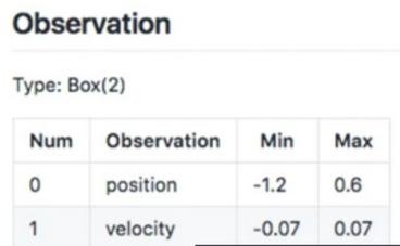
- https://github.com/openai/gym/wiki/mountaincar-v0
- https://github.com/openai/envs/mountaincar-v0
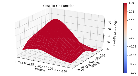
Cost-to-go Function
- Is the negative of optimal value funtion V*(s)
- what they call it in sutton & barto
- 2 state variables -> 3-D plot
Import Library
# https://deeplearningcourses.com/c/deep-reinforcement-learning-in-python
# https://www.udemy.com/deep-reinforcement-learning-in-python
from __future__ import print_function, division
from builtins import range
# Note: you may need to update your version of future
# sudo pip install -U future
#
# This takes 4min 30s to run in Python 2.7
# But only 1min 30s to run in Python 3.5!
#
# Note: gym changed from version 0.7.3 to 0.8.0
# MountainCar episode length is capped at 200 in later versions.
# This means your agent can't learn as much in the earlier episodes
# since they are no longer as long.

import gym
import os
import sys
import numpy as np
import matplotlib
import matplotlib.pyplot as plt
from mpl_toolkits.mplot3d import Axes3D
from gym import wrappers
from datetime import datetime
from sklearn.pipeline import FeatureUnion
from sklearn.preprocessing import StandardScaler
from sklearn.kernel_approximation import RBFSampler
from sklearn.linear_model import SGDRegressor

# SGDRegressor defaults:
# loss='squared_loss', penalty='l2', alpha=0.0001,
# l1_ratio=0.15, fit_intercept=True, n_iter=5, shuffle=True,
# verbose=0, epsilon=0.1, random_state=None, learning_rate='invscaling',
# eta0=0.01, power_t=0.25, warm_start=False, average=False
Feature Transformer
# Inspired by https://github.com/dennybritz/reinforcement-learning
class FeatureTransformer:
  def __init__(self, env, n_components=500):
    observation_examples = np.array([env.observation_space.sample() for x in range(10000)])
    # 4개의 밸류값의 리스트가 만개가 생긴다 in observation_examples에
    scaler = StandardScaler()
    scaler.fit(observation_examples)

    # Used to converte a state to a featurizes represenation.
    # We use RBF kernels with different variances to cover different parts of the space
    featurizer = FeatureUnion([
            ("rbf1", RBFSampler(gamma=5.0, n_components=n_components)),
            ("rbf2", RBFSampler(gamma=2.0, n_components=n_components)),
            ("rbf3", RBFSampler(gamma=1.0, n_components=n_components)),
            ("rbf4", RBFSampler(gamma=0.5, n_components=n_components))
            ])
    example_features = featurizer.fit_transform(scaler.transform(observation_examples))

    self.dimensions = example_features.shape[1]
    self.scaler = scaler
    self.featurizer = featurizer

    def transform(self, observations):
      # print "observations:", observations
      scaled = self.scaler.transform(observations)
      # assert(len(scaled.shape) == 2)
      return self.featurizer.transform(scaled)
Model
# Holds one SGDRegressor for each action
class Model:
  def __init__(self, env, feature_transformer, learning_rate):
    self.env = env
    self.models = []
    self.feature_transformer = feature_transformer
    for i in range(env.action_space.n):
      model = SGDRegressor(learning_rate=learning_rate)
      model.partial_fit(feature_transformer.transform( [env.reset()] ), [0])
      self.models.append(model)

  def predict(self, s):
    X = self.feature_transformer.transform([s])
    result = np.stack([m.predict(X) for m in self.models]).T
    assert(len(result.shape) == 2)
    return result

  def update(self, s, a, G):
    X = self.feature_transformer.transform([s])
    assert(len(X.shape) == 2)
    self.models[a].partial_fit(X, [G])

  def sample_action(self, s, eps):
    # eps = 0
    # Technically, we don't need to do epsilon-greedy
    # because SGDRegressor predicts 0 for all states
    # until they are updated. This works as the
    # "Optimistic Initial Values" method, since all
    # the rewards for Mountain Car are -1.
    if np.random.random() < eps:
      return self.env.action_space.sample()
    else:
      return np.argmax(self.predict(s))
play
def play_one(model, env, eps, gamma):
  observation = env.reset()
  done = False
  totalreward = 0
  iters = 0
  while not done and iters < 10000:
    action = model.sample_action(observation, eps)
    prev_observation = observation
    observation, reward, done, info = env.step(action)

    # update the model
    next = model.predict(observation)
    # assert(next.shape == (1, env.action_space.n))
    G = reward + gamma*np.max(next[0])
    model.update(prev_observation, action, G)

    totalreward += reward
    iters += 1

  return totalreward
Plot_cost_to_go
def plot_cost_to_go(env, estimator, num_tiles=20):
  x = np.linspace(env.observation_space.low[0], env.observation_space.high[0], num=num_tiles)
  y = np.linspace(env.observation_space.low[1], env.observation_space.high[1], num=num_tiles)
  X, Y = np.meshgrid(x, y)
  # both X and Y will be of shape (num_tiles, num_tiles)
  Z = np.apply_along_axis(lambda _: -np.max(estimator.predict(_)), 2, np.dstack([X, Y]))
  # Z will also be of shape (num_tiles, num_tiles)

  fig = plt.figure(figsize=(10, 5))
  ax = fig.add_subplot(111, projection='3d')
  surf = ax.plot_surface(X, Y, Z,
    rstride=1, cstride=1, cmap=matplotlib.cm.coolwarm, vmin=-1.0, vmax=1.0)
  ax.set_xlabel('Position')
  ax.set_ylabel('Velocity')
  ax.set_zlabel('Cost-To-Go == -V(s)')
  ax.set_title("Cost-To-Go Function")
  fig.colorbar(surf)
  plt.show()
Plot_running_avg
def plot_running_avg(totalrewards):
  N = len(totalrewards)
  running_avg = np.empty(N)
  for t in range(N):
    running_avg[t] = totalrewards[max(0, t-100):(t+1)].mean()
  plt.plot(running_avg)
  plt.title("Running Average")
  plt.show()
Main
def main(show_plots=True):
  env = gym.make('MountainCar-v0')
  ft = FeatureTransformer(env)
  model = Model(env, ft, "constant")
  gamma = 0.99

  if 'monitor' in sys.argv:
    filename = os.path.basename(__file__).split('.')[0]
    monitor_dir = './' + filename + '_' + str(datetime.now())
    env = wrappers.Monitor(env, monitor_dir)


  N = 300
  totalrewards = np.empty(N)
  for n in range(N):
    # eps = 1.0/(0.1*n+1)
    eps = 0.1*(0.97**n)
    if n == 199:
      print("eps:", eps)
    # eps = 1.0/np.sqrt(n+1)
    totalreward = play_one(model, env, eps, gamma)
    totalrewards[n] = totalreward
    if (n + 1) % 100 == 0:
      print("episode:", n, "total reward:", totalreward)
  print("avg reward for last 100 episodes:", totalrewards[-100:].mean())
  print("total steps:", -totalrewards.sum())

  if show_plots:
    plt.plot(totalrewards)
    plt.title("Rewards")
    plt.show()

    plot_running_avg(totalrewards)

    # plot the optimal state-value function
    plot_cost_to_go(env, model)


if __name__ == '__main__':
  # for i in range(10):
  #   main(show_plots=False)
  main()
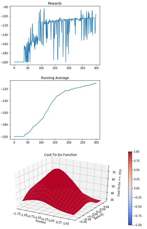
episode: 99 total reward: -113.0
eps: 0.00023311762989647067
episode: 199 total reward: -183.0
episode: 299 total reward: -96.0
avg reward for last 100 episodes: -110.08
total steps: 40586.0
Reference:
Artificial Intelligence Reinforcement Learning
RBF Networks
- RBF = Radial Basis Function
- Useful in RL
- 2 perspectives
- Linear model with feature extraction, where the feature extraction is RBF kernel
- 1-hidden layer neural network, with RBF kernel as activation function
- when we first learned about neural networks, we learned these in reverse order
- we first learned that a neural network is a nonlinear function approximator
- later, we saw that hidden units happen to learn features
RBF Basis Function
- is a non-normalized Gaussian

- x = input vector
- c = center / exemplar(模范) vector
- Only Repends on distance between x and c, not direction, hence the term radial
- Max is 1, when x == c, approaches 0 as x goes further away from c
How do we choose c?
- how many c’s should we choose?
- number of center / exemplar == number of hidden units in the RBF Network
- Each unit will have a different center
- A few different ways to choose them
Support Vecotr Machines
- SVMs also use RBF Kernels
- # of exemplars == # of training points
- in fact, with SVMs the exemplars are the training points
- this is why SVMs have fallen out of favour
- Training becomes O(N^2), prediction is O(N), N = # Training samples
- important piece of deep learning history
- SVMs were once though to be superior
Another Methods
- SVMs were once though to be superior
- Just sample a few points from the state space
- can then choose the # of exemplars
- env.observation_sapce.sample()
- how many exemplars we choose is like how many hidden units in a neural network - it’s hyperparameter that must be tuned
Implementation
- we’ll make use of sci-kit learn
- our own difect from-definition implementation would be unnecessarily slow
- RBFsampler uses a Monte Carlo algorithms(MC)
from sklearn.kernel_approximation import RBFsampler
- Standard Interface
sampler = RBFSampler()
sampler.fit(radw_data)
features = sampler.transform(raw_data)
The rest we have done before
- now that we know how to transform the raw state, the rest we should be familiar with: Q-learning, linear function approximation with gradient descent
- Unlike a feedforward neural network, the features won’t change as we learn
- exemplar we choose at the beginning will remain forever
- May seem restrictive, but works better than feedforward NN
Old Perspective vs New Perspective
- we used linear functions with polynomial features before
- now we use RBF Kernel for features
- the other Perspective: 1-hidden layer neural network
- remember that in general, this is a nonlinear transformation -> linear model at the final layer
- Recall: dot product is a cosine distance: $a^T$b = IaI IbI cos(angle(a,b))


Implementation Details
- Scale parameter(aka. Variance)
- We don’t know what’s good
- Perhaps multiple are good
- sci-kit learn has facilities that allow us to use multiple RBF samplers simultaneously
from sklearn.pipeline import FeatureUnion
- Can concatenate(连在一起的) any features, not just those from RBFSampler
- Standardize our data too:
from sklearn.preprocessing import StandardScaler
from sklearn.linear_model import SGDRegressor
# Functions:
partial_fit(X,y) # one step of gradient descent
Predict(X)
- SGDRegressor behaves a little strangely
- partial_fit() must be called at least once before we do any prediction
- Prediction must come before any real fitting, b/c we are using Q-Learning(where we need the max over Q(s,a))
- so we’ll start by calling partial_fit with dummy values
input = transform(env.reset(), target = 0)
model.partial_fit(input,target)
- after calling partial_fit(SGD) with target 0, it will make all predictions for awhile
- This is weird - a linear model shouldn’t behave this way(it may not be purely linear model)
- this quirk(怪异的性格(或行为)) is useful
- for our next task, mountain car, all rewards are -1
- therefore, Q prediction of 0 is higher than anything we can actually get
- this is the optimistic initial value method
- Technically don’t need epsilon-greedy
Prove it to ourselves
from sklearn.linear_model import SGDRegressor
model = SGDRegressor()
model.partial_fit([0,0],[0])
model.predict([[0,0]])
# array([0.]) - make sense
model.predict([0,1])
# array([0.]) - huh?
model.predict([1,0])
# array([0.]) - huh?
...
model.predict([1,1])
# array([0.]) - huh?
model.predict([99,99])
# array([0.]) - huh?
One model per action
- Another implementation detail used by Deep Q Learning too
- instead of x <- transform(s,a)
- we’ll used x <- transform(s)
- since actions are discrete, we can have a different Q(s) for every a(action)
- For mountain Car, 3 actions: left, right, nothing
- Neural Network with 3 output nodes
mountain Car
- https://github.com/openai/gym/wiki/mountaincar-v0
- https://github.com/openai/envs/mountaincar-v0
Cost-to-go Function
- Is the negative of optimal value funtion V*(s)
- what they call it in sutton & barto
- 2 state variables -> 3-D plot
Import Library
# https://deeplearningcourses.com/c/deep-reinforcement-learning-in-python
# https://www.udemy.com/deep-reinforcement-learning-in-python
from __future__ import print_function, division
from builtins import range
# Note: you may need to update your version of future
# sudo pip install -U future
#
# This takes 4min 30s to run in Python 2.7
# But only 1min 30s to run in Python 3.5!
#
# Note: gym changed from version 0.7.3 to 0.8.0
# MountainCar episode length is capped at 200 in later versions.
# This means your agent can't learn as much in the earlier episodes
# since they are no longer as long.
import gym
import os
import sys
import numpy as np
import matplotlib
import matplotlib.pyplot as plt
from mpl_toolkits.mplot3d import Axes3D
from gym import wrappers
from datetime import datetime
from sklearn.pipeline import FeatureUnion
from sklearn.preprocessing import StandardScaler
from sklearn.kernel_approximation import RBFSampler
from sklearn.linear_model import SGDRegressor
# SGDRegressor defaults:
# loss='squared_loss', penalty='l2', alpha=0.0001,
# l1_ratio=0.15, fit_intercept=True, n_iter=5, shuffle=True,
# verbose=0, epsilon=0.1, random_state=None, learning_rate='invscaling',
# eta0=0.01, power_t=0.25, warm_start=False, average=False
Feature Transformer
# Inspired by https://github.com/dennybritz/reinforcement-learning
class FeatureTransformer:
def __init__(self, env, n_components=500):
observation_examples = np.array([env.observation_space.sample() for x in range(10000)])
# 4개의 밸류값의 리스트가 만개가 생긴다 in observation_examples에
scaler = StandardScaler()
scaler.fit(observation_examples)
# Used to converte a state to a featurizes represenation.
# We use RBF kernels with different variances to cover different parts of the space
featurizer = FeatureUnion([
("rbf1", RBFSampler(gamma=5.0, n_components=n_components)),
("rbf2", RBFSampler(gamma=2.0, n_components=n_components)),
("rbf3", RBFSampler(gamma=1.0, n_components=n_components)),
("rbf4", RBFSampler(gamma=0.5, n_components=n_components))
])
example_features = featurizer.fit_transform(scaler.transform(observation_examples))
self.dimensions = example_features.shape[1]
self.scaler = scaler
self.featurizer = featurizer
def transform(self, observations):
# print "observations:", observations
scaled = self.scaler.transform(observations)
# assert(len(scaled.shape) == 2)
return self.featurizer.transform(scaled)
Model
# Holds one SGDRegressor for each action
class Model:
def __init__(self, env, feature_transformer, learning_rate):
self.env = env
self.models = []
self.feature_transformer = feature_transformer
for i in range(env.action_space.n):
model = SGDRegressor(learning_rate=learning_rate)
model.partial_fit(feature_transformer.transform( [env.reset()] ), [0])
self.models.append(model)
def predict(self, s):
X = self.feature_transformer.transform([s])
result = np.stack([m.predict(X) for m in self.models]).T
assert(len(result.shape) == 2)
return result
def update(self, s, a, G):
X = self.feature_transformer.transform([s])
assert(len(X.shape) == 2)
self.models[a].partial_fit(X, [G])
def sample_action(self, s, eps):
# eps = 0
# Technically, we don't need to do epsilon-greedy
# because SGDRegressor predicts 0 for all states
# until they are updated. This works as the
# "Optimistic Initial Values" method, since all
# the rewards for Mountain Car are -1.
if np.random.random() < eps:
return self.env.action_space.sample()
else:
return np.argmax(self.predict(s))
play
def play_one(model, env, eps, gamma):
observation = env.reset()
done = False
totalreward = 0
iters = 0
while not done and iters < 10000:
action = model.sample_action(observation, eps)
prev_observation = observation
observation, reward, done, info = env.step(action)
# update the model
next = model.predict(observation)
# assert(next.shape == (1, env.action_space.n))
G = reward + gamma*np.max(next[0])
model.update(prev_observation, action, G)
totalreward += reward
iters += 1
return totalreward
Plot_cost_to_go
def plot_cost_to_go(env, estimator, num_tiles=20):
x = np.linspace(env.observation_space.low[0], env.observation_space.high[0], num=num_tiles)
y = np.linspace(env.observation_space.low[1], env.observation_space.high[1], num=num_tiles)
X, Y = np.meshgrid(x, y)
# both X and Y will be of shape (num_tiles, num_tiles)
Z = np.apply_along_axis(lambda _: -np.max(estimator.predict(_)), 2, np.dstack([X, Y]))
# Z will also be of shape (num_tiles, num_tiles)
fig = plt.figure(figsize=(10, 5))
ax = fig.add_subplot(111, projection='3d')
surf = ax.plot_surface(X, Y, Z,
rstride=1, cstride=1, cmap=matplotlib.cm.coolwarm, vmin=-1.0, vmax=1.0)
ax.set_xlabel('Position')
ax.set_ylabel('Velocity')
ax.set_zlabel('Cost-To-Go == -V(s)')
ax.set_title("Cost-To-Go Function")
fig.colorbar(surf)
plt.show()
Plot_running_avg
def plot_running_avg(totalrewards):
N = len(totalrewards)
running_avg = np.empty(N)
for t in range(N):
running_avg[t] = totalrewards[max(0, t-100):(t+1)].mean()
plt.plot(running_avg)
plt.title("Running Average")
plt.show()
Main
def main(show_plots=True):
env = gym.make('MountainCar-v0')
ft = FeatureTransformer(env)
model = Model(env, ft, "constant")
gamma = 0.99
if 'monitor' in sys.argv:
filename = os.path.basename(__file__).split('.')[0]
monitor_dir = './' + filename + '_' + str(datetime.now())
env = wrappers.Monitor(env, monitor_dir)
N = 300
totalrewards = np.empty(N)
for n in range(N):
# eps = 1.0/(0.1*n+1)
eps = 0.1*(0.97**n)
if n == 199:
print("eps:", eps)
# eps = 1.0/np.sqrt(n+1)
totalreward = play_one(model, env, eps, gamma)
totalrewards[n] = totalreward
if (n + 1) % 100 == 0:
print("episode:", n, "total reward:", totalreward)
print("avg reward for last 100 episodes:", totalrewards[-100:].mean())
print("total steps:", -totalrewards.sum())
if show_plots:
plt.plot(totalrewards)
plt.title("Rewards")
plt.show()
plot_running_avg(totalrewards)
# plot the optimal state-value function
plot_cost_to_go(env, model)
if __name__ == '__main__':
# for i in range(10):
# main(show_plots=False)
main()
episode: 99 total reward: -113.0
eps: 0.00023311762989647067
episode: 199 total reward: -183.0
episode: 299 total reward: -96.0
avg reward for last 100 episodes: -110.08
total steps: 40586.0
Reference:
Artificial Intelligence Reinforcement Learning


Comments