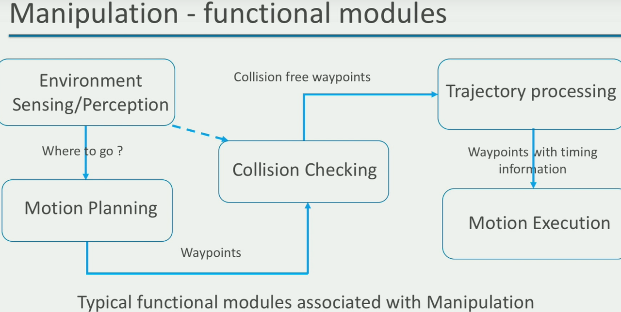
ROS Manipulation Overview

• Moveit! - a ROS package for manipulation
• Moveit! setup assistant - configure robot setups to use moveit
• plan and execute motion - the “Move_group” Ros Node
• Implement a simple pick and place pipeline
• interact with the environment and modify it using a robot to perform useful tasks
  • pick and place an object
  • fasten two parts of a car chassis
• An integral part of automation

• Moveit : open source software library for manipulation
  • easy integration with ros
  • maintain information consistency
  • integrate robot kinematic information with planning
  • report and request alternative motion plans in case of collisions
  • Account for any hardware limitations such as joint limits
  • keep track of the current state of the robot and its environment while performing a manipulation task
  • talk to the robot hardware/simulation and notify the ros application once a desired manipulation task is complete
• Moveit! - from a user’s perspective
  • move_group Ros node
    • several ros Service and actions (APIs)
    • Configuring the move_group node
      • robot description (URDF/XACRO)
      • robot_semantic description(SRDF)
      • joint limit, planner
• where are trajectories executed
  • simulated robot or real hardware
• what controls trajectory execution in simulation or hardware
  • controller on a simulator or a hardware driver
  • simulation package hrwros_gazebo
• how does moveit! talk to the controllers from simulation?
  • ros topics and actions servers

Basic commands

command

#!/bin/bash
rosrun moveit_commander moveit_commander_cmdline.py /joint_states:=/combined_joint_states joint_states:=/combined_joint_states

• list all usable command
  • help
• select the “group” to use
  • use
• plan and execute motion form srdf
  • go
• get current joint state and pose
  • current
• Execute multiple commands
  • load <path_to_script_file/scrip_file_name>

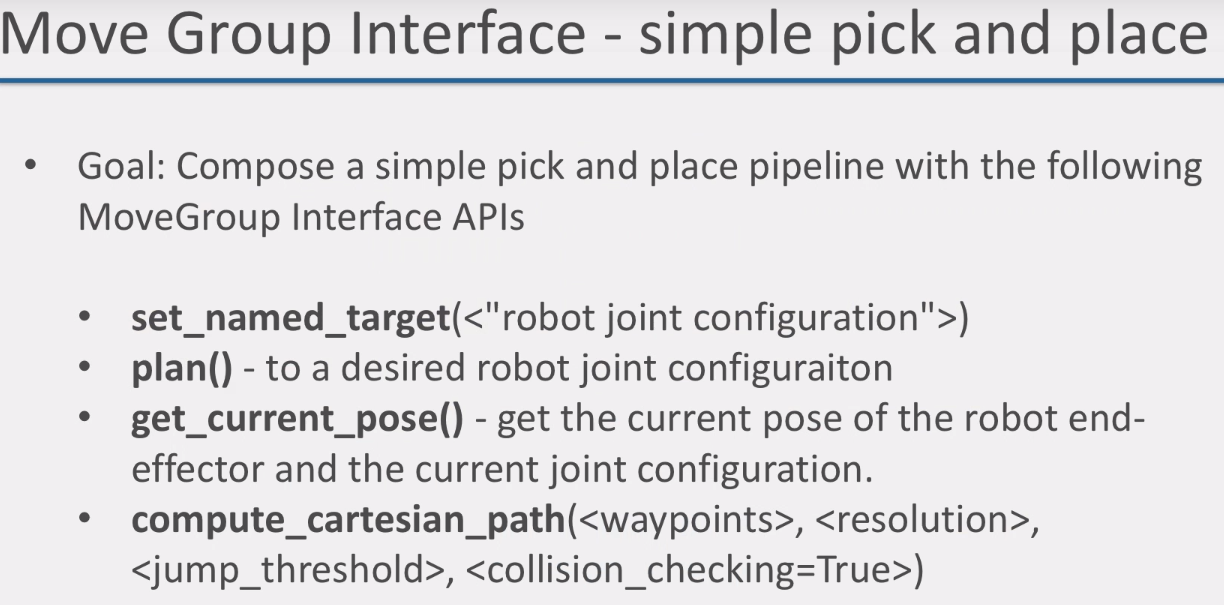
MoveGroup Interface

• A collection of APIs to access the various capabilities of Move_group Ros node
• Create Moveit!-based ROS applications
• Setup a simple pick and plcae pipline in code with movegroup APIs
  • using ROS action client

TF2 ROS Introduction

• command line tool
  • tf_echo(static)

example

tf tf_echo world robot2_pedestal_link

• tf2_ros package
  • implement functional aspects, and actively maintain relations
  • Transform Pose: allows for “time travel” - look up the spatiotemporal時空 relation
• was there a TF(1) package?
  • yes
  • used in many applications
  • command line tools
  • All in one (vs clear separation in TF2)
• All TF functionalities are migrated to tf2_ros
  • availability of a transform buffer in tf2_ros
• Information representation
  • Quantification
    • 3D Transfromation

    • ROS topic: /tf (tf2_msgs/TFMessage)

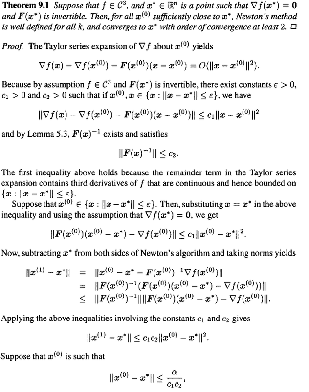
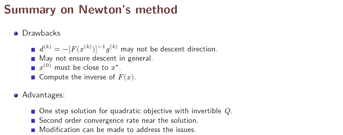
1. Features of Newton’s method

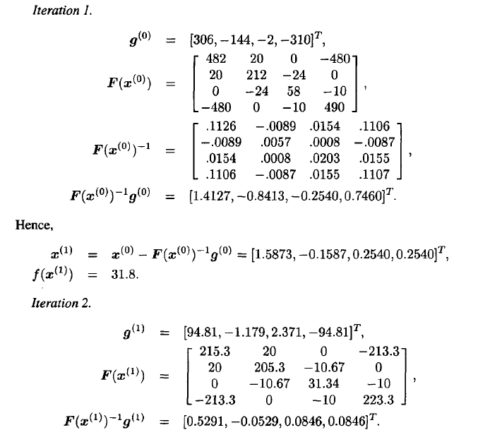
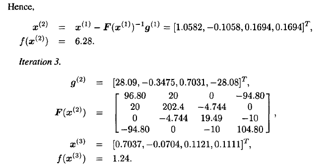
• Use both first and second derivatives.
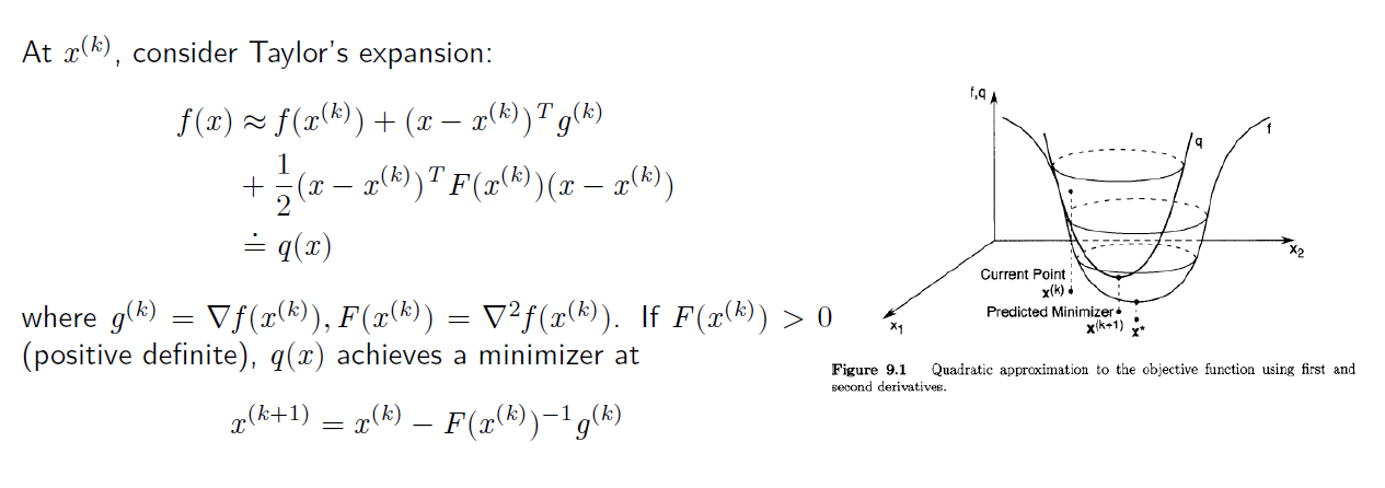
• Based on local quadratic approximation to the objective function.
• Requires a positive Hessian to work.
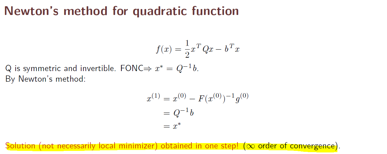
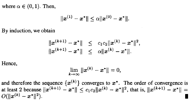
• Converge quadratically under conditions.

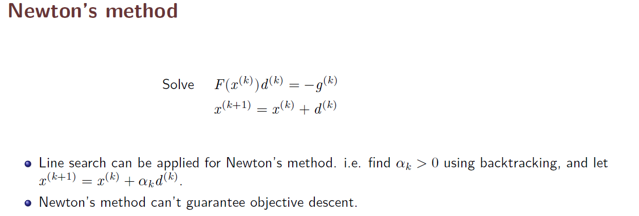
2. Derivation of Newton’s method

• Rate of convergence is a measure of how fast the difference between the solution point and its estimates goes to zero. Faster algorithms usually use second-order information about the problem functions when calculating the search direction.

3. Two issues for Newton’s method

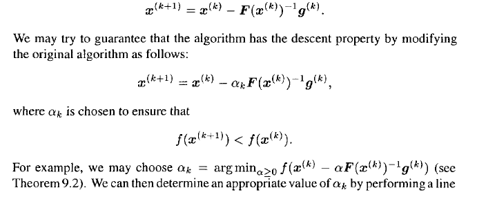
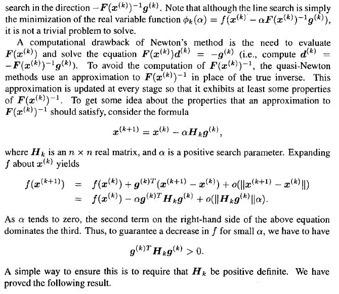
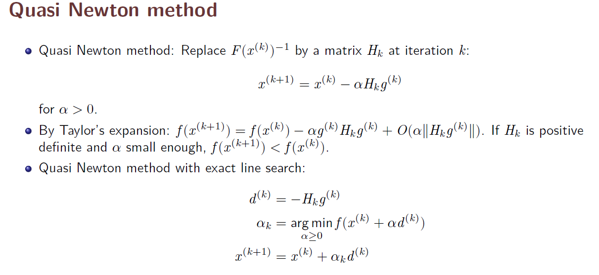
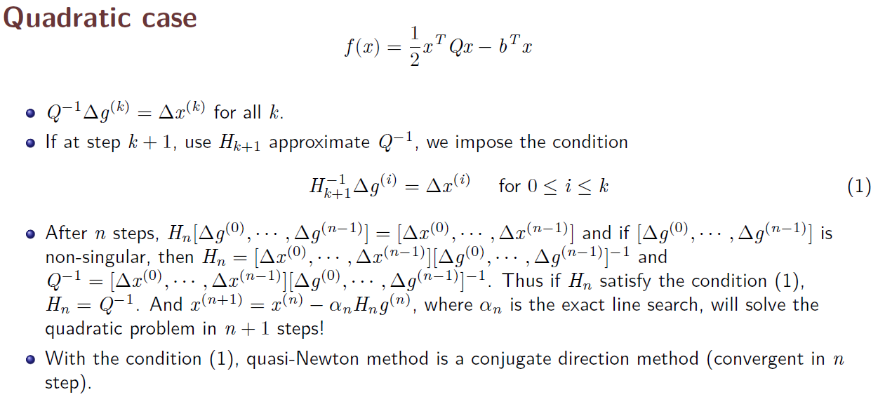
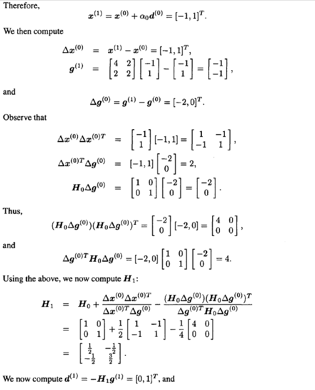
• When the dimension n is large, obtain F(x^(k)) and its inverse is computationally expensive => consider quasi-newton’s method
• Indefinite Hessian: the direction is not necessarily descending

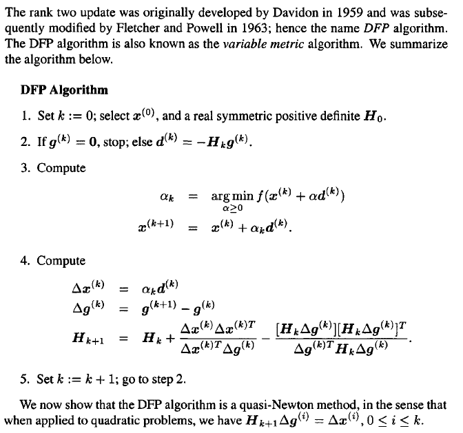
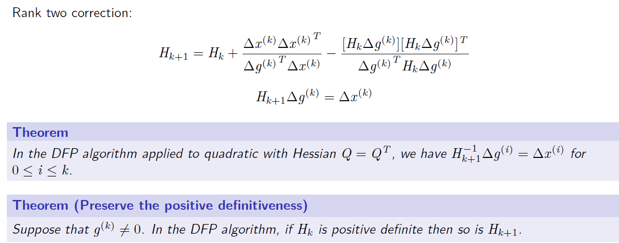
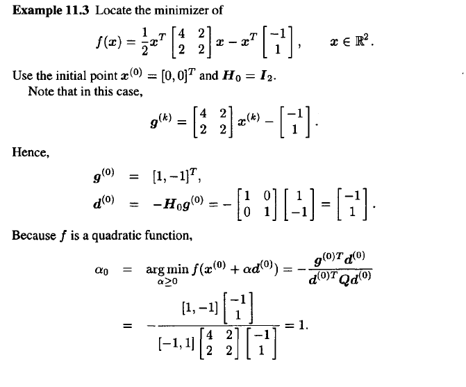
4. Quasi Newton Method

• Big O notation is a mathematical notation that describes the limiting behavior of a function when the argument tends towards a particular value or infinity.
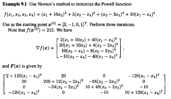
• Newton’s method is one of the more successful algorithms for optimization
• If it converges, it has a quadratic order of convergence.
• However, as pointed out before, for a general nonlinear objective function, convergence to a solution cannot be guaranteed from an arbitrary initial point x^(0). In general, if the initial point is not sufficiently close to the solution, then the algorithm may not possess the descent property
• Recall that the idea behind Newton’s method is to locally approximate the function f being minimized, at every iteration, by a quadratic function. The minimizer for the quadratic approximation is used as the starting point for the next iteration
• This leads to Newton’s recursive algorithm

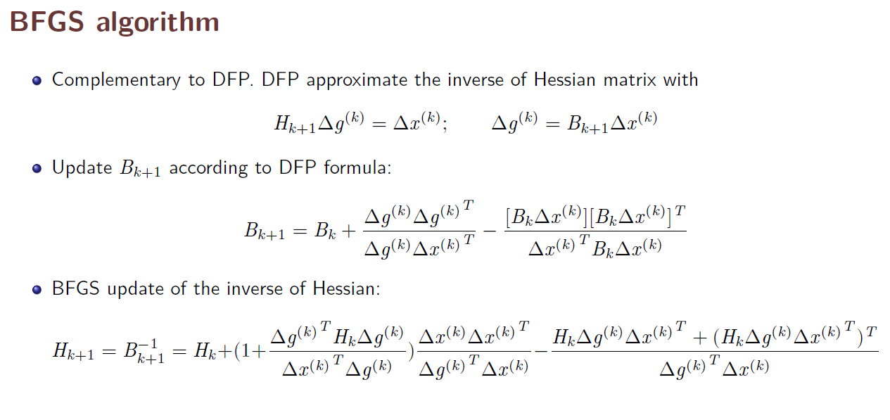
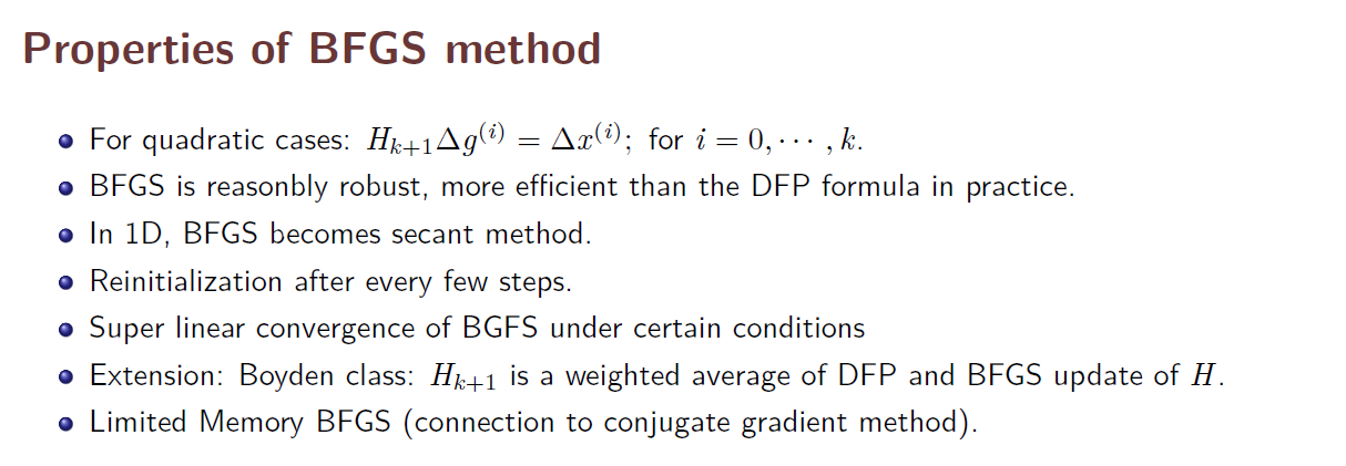
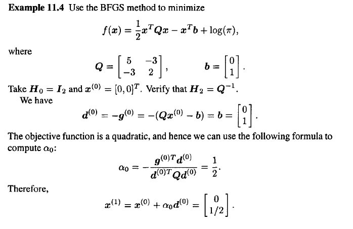
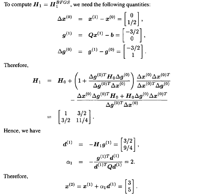
5. THE BFGS ALGORITHM

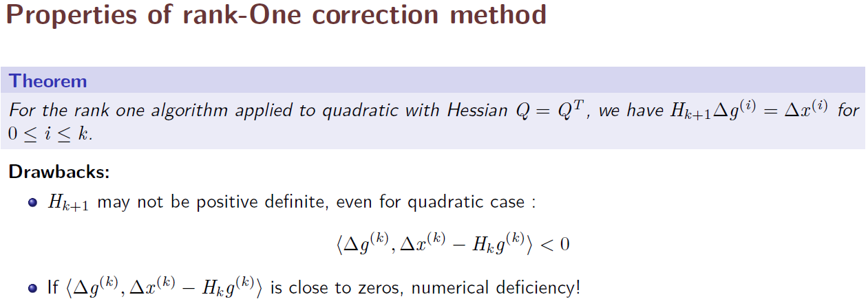
• In 1970, an alternative update formula was suggested independently by Broyden, Fletcher, Goldfarb, and Shanno. The method is now called the BFGS algorithm, which we discuss in this section
• In numerical optimization, the Broyden–Fletcher–Goldfarb–Shanno (BFGS) algorithm is an iterative method for solving unconstrained nonlinear optimization problems

Optimization method - Standford University

https://www.youtube.com/results?search_query=convex+function

TD(λ)

• Generalize N-step method
• λ is associated with something called the []”eligibility trace”(전격 흔적)](https://sumniya.tistory.com/14)
  • eligibility trace라는 개념 : 이는 과거에 방문했던 state 중에서 현재 얻게 되는 reward에 영향을 주는 state를 판단하여, 현재 얻게 되는 reward을 해당 state에 나누어주는 것입니다. 이때, 영향을 주었다고 판단하는 index를 credit이라고하고 이 credit을 assign할 때, 두 가지 기준을 씁니다. 1) Frequency heuristic(얼마나 자주 방문했는가?) 2) Recency heuristic(얼마나 최근에 방문 했는가?)
• N-step method code is complicated - not trivial to keep track of all rewards(then flush them once episode is over)
• TD(λ) allows us a more elegant method to trade-off between TD(0) and MC
• can update after just 1 step
• λ = 0 gives us TD(0), λ=1 gives us Monte Carlo

  N-step method

• Recall:

• strange idea: combine these :

TD(λ)

• let’s take this strangeness to the next level - let’s combine more G’s, even an infinite number of G’s

• λ must sum to 1 so that the result is on the same scale as individual G’s
• in TD(λ). we make the coefficients decrease geometrically

• Problem: these don’t sum to 1
• we are most interested in the case when n - > ∞
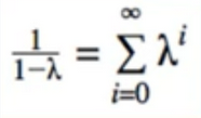
• we know this from calculus:

• therefore, we should scale the sum by thins amount
• we call this the **

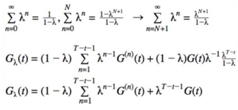
• we assume our episode will end at some point(say, time step T)
• when we reach step T - t, the episode is over, so any N-step return beyond this is the Full MC return, G(t)
• separate the partial N-step returns and the full returns

• manipulate 2nd term to simplify the sum

• simplify further

• when λ=0, we get the TD(0) return since $0^0$ = 1
• when λ=1, we get the full return(MC)
• any λ between 0 and 1 gives us a combination of individual returns(with geometrically decreasing weight)

• isn’t this much more computational effort than both MC and N-step methods?
• yes, we would need to calculate G(t), $G^1$(t),…,$G^t$(t)
• lots of work (benefit is not clear)
• the algorithm we’re about to learn is an approximation to calculate the true λ-return(since that would be computationally infeasible)

TD(0)

• let’s go back to TD(0) for a moment
• we call target - prediction the TD error

• parameter update is still gradient descent

• Eligibility trace is a vector the same size as parameter vector:

• Eligibility Trace/ vector keeps track of old gradients, much like momentum from deep learning
• λ tell us “how much” of the past we want to keep
  • $e_0$ = 0, $e_t$ = $∇0$V($s_t$) + ɣλe(t_1)

back to TD(λ)

• redefine the parameter update to use e instead of only gradient

• recall how momentum works
• update only depends on next state
• we can do updates in 1 step rather than waiting N steps
• but still, just an approximation to using true λ-return
• N-step method and true λ-return require waiting for future rewards
  • we call this the “forward view”
• in TD(λ), we update the current param based on past errors
  • we call this the “backward view”

Code

# https://deeplearningcourses.com/c/deep-reinforcement-learning-in-python
# https://www.udemy.com/deep-reinforcement-learning-in-python
from __future__ import print_function, division
from builtins import range
# Note: you may need to update your version of future
# sudo pip install -U future
#
# Note: gym changed from version 0.7.3 to 0.8.0
# MountainCar episode length is capped at 200 in later versions.
# This means your agent can't learn as much in the earlier episodes
# since they are no longer as long.
#
# Adapt Q-Learning script to use TD(lambda) method instead

import gym
import os
import sys
import numpy as np
import matplotlib.pyplot as plt
from gym import wrappers
from datetime import datetime

# code we already wrote
from q_learning import plot_cost_to_go, FeatureTransformer, plot_running_avg

Base model

class BaseModel:
    # this is eligience traces
  def __init__(self, D):
    self.w = np.random.randn(D) / np.sqrt(D)

  def partial_fit(self, input_, target, eligibility, lr=1e-2):
    self.w += lr*(target - input_.dot(self.w))*eligibility

  def predict(self, X):
    X = np.array(X)
    return X.dot(self.w)

model

# Holds one BaseModel for each action
class Model:
  def __init__(self, env, feature_transformer):
    self.env = env
    self.models = []
    self.feature_transformer = feature_transformer

    D = feature_transformer.dimensions # 2000 D
    self.eligibilities = np.zeros((env.action_space.n, D))
    for i in range(env.action_space.n):
      model = BaseModel(D)
      self.models.append(model)

  def predict(self, s):
    X = self.feature_transformer.transform([s])
    assert(len(X.shape) == 2)
    result = np.stack([m.predict(X) for m in self.models]).T
    assert(len(result.shape) == 2)
    return result

  def update(self, s, a, G, gamma, lambda_):
    X = self.feature_transformer.transform([s])
    assert(len(X.shape) == 2)
    self.eligibilities *= gamma*lambda_
    self.eligibilities[a] += X[0]
    self.models[a].partial_fit(X[0], G, self.eligibilities[a])

  def sample_action(self, s, eps):
    if np.random.random() < eps:
      return self.env.action_space.sample()
    else:
      return np.argmax(self.predict(s))

play

# returns a list of states_and_rewards, and the total reward
def play_one(model, env, eps, gamma, lambda_):
  observation = env.reset()
  done = False
  totalreward = 0
  iters = 0
  # while not done and iters < 200:
  while not done and iters < 10000:
    action = model.sample_action(observation, eps)
    prev_observation = observation
    observation, reward, done, info = env.step(action)

    # update the model
    next = model.predict(observation)
    assert(next.shape == (1, env.action_space.n))
    G = reward + gamma*np.max(next[0])
    model.update(prev_observation, action, G, gamma, lambda_)

    totalreward += reward
    iters += 1

  return totalreward

main

if __name__ == '__main__':
  env = gym.make('MountainCar-v0')
  ft = FeatureTransformer(env)
  model = Model(env, ft)
  gamma = 0.9999
  lambda_ = 0.7

  if 'monitor' in sys.argv:
    filename = os.path.basename(__file__).split('.')[0]
    monitor_dir = './' + filename + '_' + str(datetime.now())
    env = wrappers.Monitor(env, monitor_dir)


  N = 300
  totalrewards = np.empty(N)
  costs = np.empty(N)
  for n in range(N):
    # eps = 1.0/(0.1*n+1)
    eps = 0.1*(0.97**n)
    # eps = 0.5/np.sqrt(n+1)
    totalreward = play_one(model, env, eps, gamma, lambda_)
    totalrewards[n] = totalreward
#     print("episode:", n, "total reward:", totalreward)
  print("avg reward for last 100 episodes:", totalrewards[-100:].mean())
  print("total steps:", -totalrewards.sum())

  plt.plot(totalrewards)
  plt.title("Rewards")
  plt.show()

  plot_running_avg(totalrewards)

  # plot the optimal state-value function
  plot_cost_to_go(env, model)

TD LAMDA summary

• we learned techniques that can be applied anywhere we would use Qlearning or SARSA
• general tools that we can test in a variety of situations
• “technically” got more practice with RBF networks too

N-step Methods

• we saw how N-step methods provide a “bridge” between TD(0) and MC
• we saw that we can combine all the N-step returns
• this gives us the λ-return
• we saw that λ=0 gives us TD(0). λ=1 gives us MC

Eligibility Traces

• we looked at the use of eligibility traces to approximate TD(λ) using the true λ-return(since actually calculating it would be lots of effort)
• we saw that it looks a lot like deep learning momentum
• new tools for our toolbox
• not guaranteed that any particular algorithm will work for our problem, but more tools = more thing to try

``` Reference:

Artificial Intelligence Reinforcement Learning

Advance AI : Deep-Reinforcement Learning

Cutting-Edge Deep-Reinforcement Learning

ROS Navigation stack

• 2D Navigation
• inputs:
  • Odometry
  • Sensor data
  • Goal Pose
• Output:
  • safe velocity commands
• only for differential drive or holonomic wheeled robots
• requires a planar laser
• performs best on square or circular robots
• ROS topics : Transport information between nodes

Move_base

• provides an implementation of an action
  • Actions are used for long term tasks
• Uses a global and local planner to accomplish its global navigation goal
• Manages communication between the components of the navigation stack

Rviz

1. Under Global options on the left side panel for fixed frame, change base_link or base_footprint to Odom
2. click on Add and select the by topic tab
3. choose odometry and click on OK

Navigation necessary

1. Map of the environment
   • use a pre-existing map
   • built by the robot itself during a mapping process
   • this process is called SLAM
     • “gmapping”
   • simultaneous Localization and mapping
   • it gathers information about the environment using laser scanning
2. Localization
   • Global methods
   • GPS accuracy ~3.5m
   • Wi-Fi hotspot accuracy ~40m
   • cell towers accuracy ~600m - Local methods
   • laser can accuracy ~5cm
   • cameras accuracy ~10cm
3. Path planning
4. Obstacle avoidance

Exercise

Create unknown_obstacle.py

#!/usr/bin/env python
import rospy
import os
# Import the spawn urdf model service from Gazebo.
from gazebo_msgs.srv import SpawnModel, SpawnModelRequest, GetModelProperties, GetModelPropertiesRequest
from geometry_msgs.msg import Pose

def spawn_unknown_obstacle(obstacle_name, obstacle_model_xml, obstacle_pose):
  # Service proxy to spawn urdf object in Gazebo.
  spawn_obstacle_service = rospy.ServiceProxy('/gazebo/spawn_urdf_model', SpawnModel)
  # Create service request.
  spawn_obstacle_request = SpawnModelRequest()
  spawn_obstacle_request.model_name = obstacle_name
  spawn_obstacle_request.model_xml = obstacle_model_xml
  spawn_obstacle_request.robot_namespace = ''
  spawn_obstacle_request.initial_pose = obstacle_pose
  spawn_obstacle_request.reference_frame = 'map'
  # Call spawn model service.
  spawn_obstacle_response = spawn_obstacle_service(spawn_obstacle_request)
  if(not spawn_obstacle_response.success):
    rospy.logerr('Could not spawn unknown obstacle')
    rospy.logerr(spawn_obstacle_response.status_message)
  else:
    rospy.loginfo(spawn_obstacle_response.status_message)

def check_obstacle_existence(obstacle_name):
  # Service proxy to spawn urdf object in Gazebo.
  check_obstacle_service = rospy.ServiceProxy('/gazebo/get_model_properties', GetModelProperties)

  check_obstacle_response = check_obstacle_service(obstacle_name)
  return check_obstacle_response.success


if __name__ == '__main__':
  try:
    # Initialize a ROS Node
    rospy.init_node('spawn_unknown_obstacle')
    #Get file name of the object to be spawned.
    with open(os.path.join(os.environ["HOME"], "hrwros_ws/src/hrwros_support/urdf/unknown_obstacle/unknown_obstacle.urdf"), "r") as box_file:
      box_xml = box_file.read()
    # Wait for a couple of seconds to prevent the unknown obstacle from being
    # considered as a part of the map.
    rospy.sleep(4)

    if not check_obstacle_existence('unknown_obstacle1'):
      # First obstacle.
      obstacle1_pose = Pose()
      obstacle1_pose.position.x = -1.0
      obstacle1_pose.position.y = 1.2
      obstacle1_pose.position.z = 0.0
      obstacle1_pose.orientation.x = 0.0
      obstacle1_pose.orientation.y = 0.0
      obstacle1_pose.orientation.z = 0.0
      obstacle1_pose.orientation.w = 1.0
      spawn_unknown_obstacle('unknown_obstacle1', box_xml, obstacle1_pose)

    if not check_obstacle_existence('unknown_obstacle2'):
      # Second obstacle.
      obstacle2_pose = Pose()
      obstacle2_pose.position.x = -1.0
      obstacle2_pose.position.y = 3.0
      obstacle2_pose.position.z = 0.0
      obstacle2_pose.orientation.x = 0.0
      obstacle2_pose.orientation.y = 0.0
      obstacle2_pose.orientation.z = 0.0
      obstacle2_pose.orientation.w = 1.0
      spawn_unknown_obstacle('unknown_obstacle2', box_xml, obstacle2_pose)

  except rospy.ROSInterruptException:
    rospy.loginfo("Interrupt received to stop ROS node.")

move.py

#!/usr/bin/env python
import rospy
import sys
# Brings in the SimpleActionClient
import actionlib
from actionlib_msgs.msg import GoalStatus

# Brings in the messages used by the MoveBase action, including the
# goal message and the result message.
from move_base_msgs.msg import MoveBaseAction, MoveBaseGoal, MoveBaseResult, MoveBaseActionResult

if __name__ == '__main__':
    try:
        # Initialize a ROS Node
        rospy.init_node('move_turtlebot')
        # Create a SimpleActionClient for the move_base action server.
        turtlebot_navigation_client = actionlib.SimpleActionClient('move_base', MoveBaseAction)
        # Wait until the move_base action server becomes available.
        rospy.loginfo("Waiting for move_base action server to come up...")
        turtlebot_navigation_client.wait_for_server()
        rospy.loginfo("move_base action server is available...")
        # Creates a goal to send to the action server.
        turtlebot_robot1_goal = MoveBaseGoal()
        # Construct the target pose for the turtlebot in the "map" frame.
        turtlebot_robot1_goal.target_pose.header.stamp = rospy.Time.now()
        turtlebot_robot1_goal.target_pose.header.frame_id = "map"
        turtlebot_robot1_goal.target_pose.header.seq = 1
        turtlebot_robot1_goal.target_pose.pose.position.x = 2
        turtlebot_robot1_goal.target_pose.pose.position.y = 1
        turtlebot_robot1_goal.target_pose.pose.position.z = 0.0
        turtlebot_robot1_goal.target_pose.pose.orientation.x = 0.0
        turtlebot_robot1_goal.target_pose.pose.orientation.y = 0.0
        turtlebot_robot1_goal.target_pose.pose.orientation.z = 0.0
        turtlebot_robot1_goal.target_pose.pose.orientation.w = 1.0
        # Send the goal to the action server.
        turtlebot_navigation_client.send_goal(turtlebot_robot1_goal)
        rospy.loginfo("Goal sent to move_base action server.")
        # Wait for the server to finish performing the action.
        turtlebot_navigation_client.wait_for_result()
        # Display a log message depending on the navigation result.
        navigation_result_status = turtlebot_navigation_client.get_state()
        if GoalStatus.SUCCEEDED != navigation_result_status:
            rospy.logerr('Navigation to the desired goal failed :(. Sorry, try again!)')
        else:
            rospy.loginfo('Hooray! Successfully reached the desired goal!')
    except rospy.ROSInterruptException:
        rospy.loginfo("Interrupt received to stop ROS node.")