for Robot Artificial Inteligence

8. Gradient Methods

|

1. Gradient Methods Introduction

  • we consider a class of search methods for real-valued functions on $R^n$
  • we use terms like level sets, normal vectors, tangent vectors, and so on
  • Recall that a level set of a function f:$R^n$ -> R is the set of points x satisfying f(x) = c for some constant c.
  • simple and intuitive
  • every iteration is inexpensive
  • does not require second derivatives
  • extensions: nonsmooth optimization, combining with duality splitting, coordinate descent, alternating direction, stochastic, online learning
  • suitable for large-scale problem, parallelization

2. Geometric interpretation of gradients and gradient descent

  • ∇f($x_0$),if it is not zero, is orthogonal to the tangent of the level set curves of f passing $x_0$ on the level set f(x) = c, point outward(点向外)
  • Thus, the direction of maximum rate of increase of a real-valued differentiable function at a point is orthogonal to the level set of the function through that point.
  • In other words, the gradient acts in such a direction that for a given small displacement, the function f increases more in the direction of the gradient than in any other direction
  • To prove this statement, recall that <∇f(x),d>, IIdII = 1, is the rate of increase of f in the direction d at the point x By the Cauchy-Schwarz inequality,

  • Thus, the direction in which ∇f(x) points the direction of maximum rate of increase of f at x.
  • The direction in which —∇f(x) points is the direction of maximum rate of decrease of f at x.
  • Hence, the direction of negative gradient is a good direction to search if we want to find a function minimizer

  • We refer to the above as a gradient descent algorithm (or simply a gradient algorithm).
  • The gradient varies as the search proceeds, tending to zero as we approach the minimizer.
  • We have the option of either taking very small steps and re-evaluating the gradient at every step, or we can take large steps each time.
  • The first approach results in a laborious method of reaching the minimizer, whereas the second approach may result in a more zigzag path to the minimizer.

  • The advantage of the second approach is a possibly fewer number of the gradient evaluations.
  • Among many different methods that use the above philosophy(思想体系) the most popular is the method of steepest descent
  • Gradient methods are simple to implement and often perform well.

3. Descent direction

4. Classical Gradient Method

  • Small stepsizes: iterations are more likely converge, but it might requires more iteration and thus evaluations of ∇f
  • Large step sizes: better use of ∇f(x) and it may reduce the total number of iterations, but it can cause oversmoothing and zig-zags which lead to divergent iterations
  • Choice of stepsizes: fixed: k constant; 1D line search (backtracking, exact, Barzilai-Borwein with nonmonotone line search)

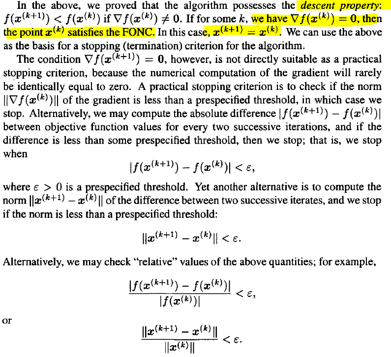
5. Stopping Criteria

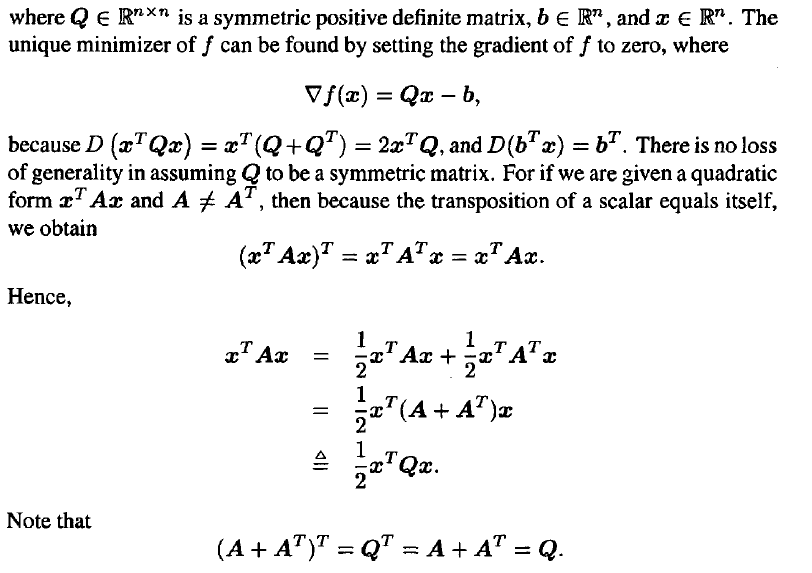
6. Calculation of Gradients

  • Analytic form: use pen and paper or Mathematica/Matlab

7. The method of steepest descent

  • Also known as gradient descent with exact line search
  • The method of steepest descent is a gradient algorithm where the step size $α_k$ is chosen to achieve the maximum amount of decrease of the objective function at each individual step.
  • Stepsize $α_k$ is determined by

  • For quadratic program, $α_k$ has closed form.
  • For problem with inexpensive evaluation values but expensive gradient evaluations
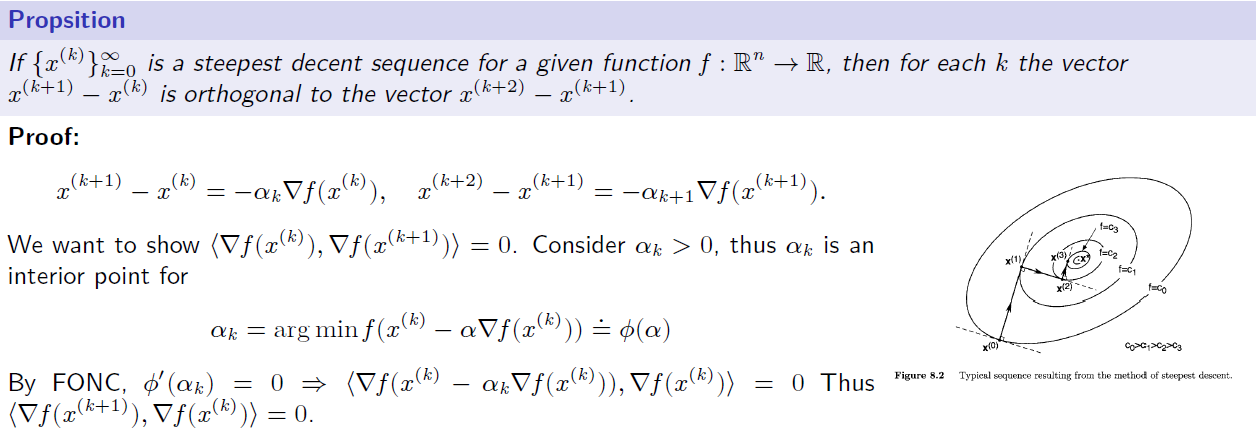
  • To summarize, the steepest descent algorithm proceeds as follows: at each step, starting from the point $x^k$, we conduct a line search in the direction -∇f($x^k$) until a minimizer, x^(k+1),is found.

8. orthogonality

9. Function Decreasing

  • relative(比较的)

10. Steepest descent for quadratic programming

11. Convergence for quadratic programming

  • The method of steepest descent is an example of an iterative algorithm.
  • This means that the algorithm generates a sequence of points, each calculated on the basis of the points preceding it.
  • The method is a descent method because as each new point is generated by the algorithm, the corresponding value of the objective function decreases in value (i.e., the algorithm possesses the descent property).
  • We say that an iterative algorithm is globally convergent if for any arbitrary starting point the algorithm is guaranteed to generate a sequence of points converging to a point that satisfies the FONC for a minimizer.
  • When the algorithm is not globally convergent, it may still generate a sequence that converges to a point satisfying the FONC, provided the initial point is sufficiently close to the point.
  • In this case, we say that the algorithm is locally convergent.
  • How close to a solution point we need to start for the algorithm to converge depends on the local convergence properties of the algorithm.
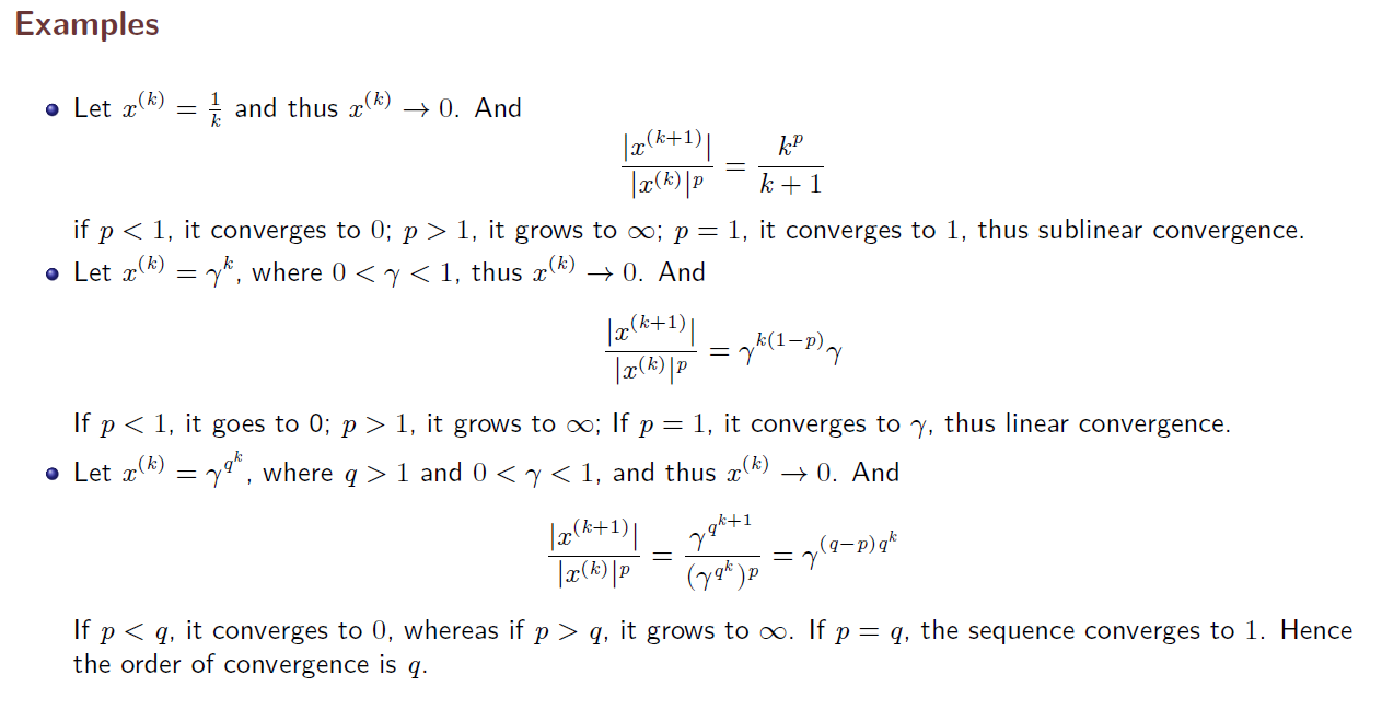
  • related issue of interest pertaining to a given locally or globally convergent algorithm is the rate of convergence; that is, how fast the algorithm converges to a solution point.

https://www.youtube.com/results?search_query=convex+function

Comment  Read more

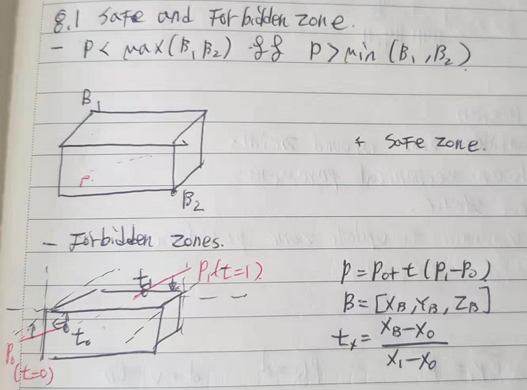
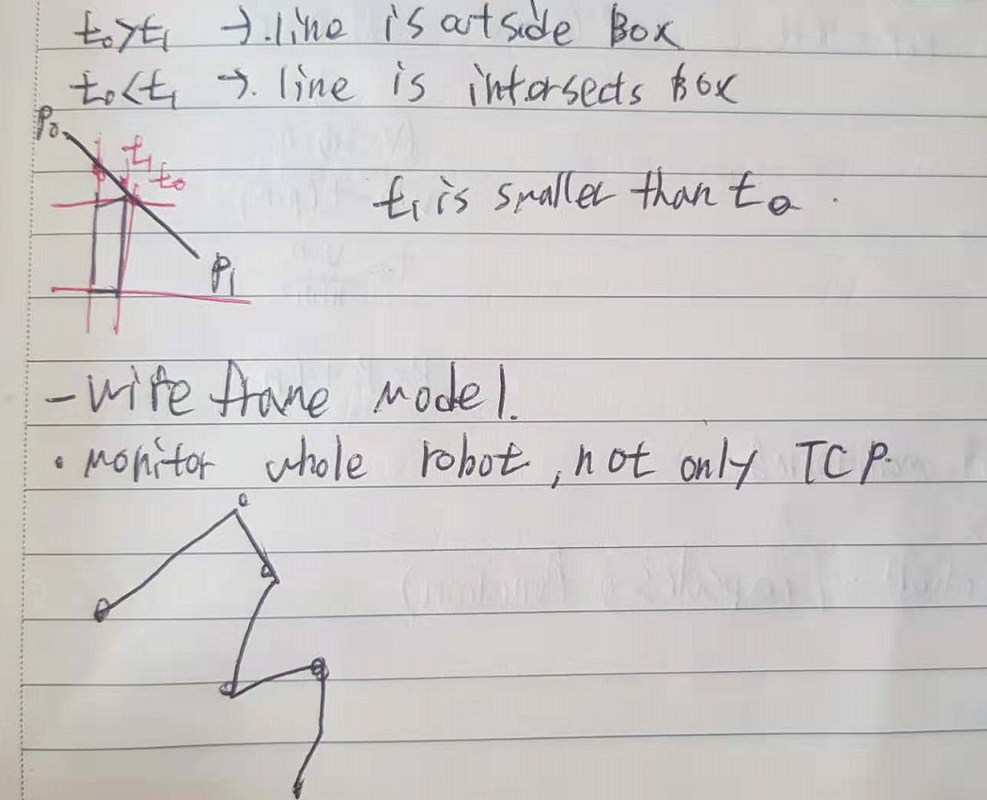
7. Work space Monitoring

|

Work space monitoring

  • Restrict the working space of the robot for safety reason
    • Safe zone, Forbidden zone
  • Collision predicted at planning time
  • Movement can be absorbed before it start
  • Use cuboids(矩形体:직육면체) for simplicity
  • Linearize movements(segmentation)

1. Safe and forbidden zone

2.Self Collision

  • Generate forbidden zone around Joints
  • Size depends on mechanical parameters
  • zones are not static
  • use direct kinematics to update zone position

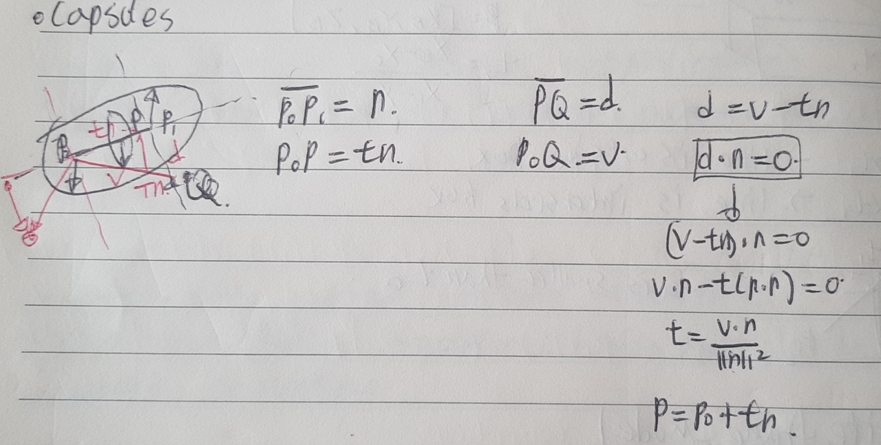
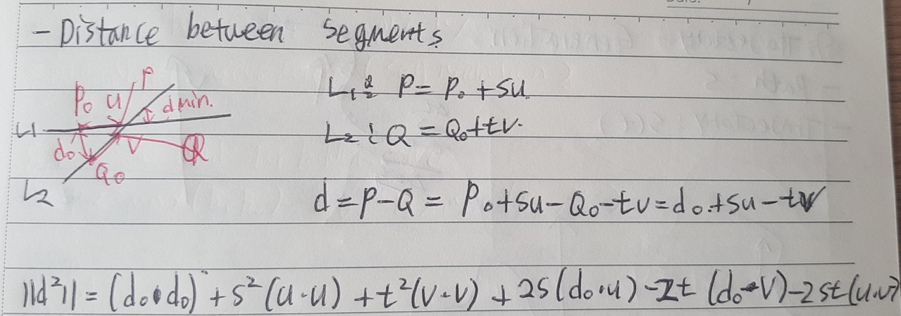
3. Multi-Robot Monitoring

  • Exclusive zones
  • collision detection (capsules functions)

Comment  Read more

7. URDF

|

URDF - Overview

  • limitation of URDF
    • robot descriptions cannot be changed
    • only tree structures
    • No
    • Low reusability of URDFs
  • Limitation 1 - immutability(불변성)
    • result of typical control flow
    • robot description read only once from parameter server
    • no standardized way to notify consumers of changes
    • risk of desynchronization of nodes
  • Limitation 2 - no cycles
    • joints have only a single parent and child
    • only acyclic(비순환적인), directed graphs(or:trees) can be modeled
    • Real-world impact: dual-arm manipulation, parallel grippers, etc
  • Limitation3 - reusability
    • Only a single tag in a URDF
    • No support for import of remote files
    • Composite scenes have to be merged manually
    • No way to compose multiple URDFs
  • Solution: Xacro(XML Macros)
    • Programmatic URDF generation
    • Templates
    • Parameters
  • Xacro:Composability(결합성)?
    • Import macros from other files
    • paramerize templates
    • composite robots & scenes easier:
      • import macro from file
      • invoke macro

        URDF

  • Defined the structure of the robot
    • link
    • joint
  • Defined basic geometry
    • Box
  • Update the dimensions
  • specify a color
  • place it on the floor
  • put it in the right location
  • Adjust the size the shape
  • Raise the object so that it rests on the floor
  • change the color
  • update its location
  • the default origin for primitive shapes is the center of the shape, which means that the box is half sunk into the floor. to fix this, the z offset the origin needs to be changed to half the height of the object
  • to change the location of the object, the offset from the world needs to be redefined. this is done by changing the x and y coordinates of the “origin” element within the joint that connects the object to the world

object create Step

  1. Import the model definition(xacro macro)
  2. Add the model to the factory(instantiation)
  3. fixating(정착시키다) it in place(joint)
  4. updating orientation
  5. the import statement consists of a few parts:
    • the xacro:include statement itself
    • the filename attribute specifying the name of the file to import(using a package relative path)
  6. Finally, we also need to add the macro cell, which will actually instantiate(예시) the model. to prevent nameclashes, we’ll configure the new object to use a unique “prefix”
    • to connect the robot to factory we will connect it to the pedestal rather than the world itself.
    • this is so that if the pedestal ever need to be moved, the robot will move with it, rather than having to update the robot’s position manually. this is done by specifying the parent in the joint as the pedestal and the child as the robot
    • finally, the orientation needs to be corrected. this is done by adding an rpy attribute to the origin element that specifies the orientation.
    • As Ros uses radian for angles, we’ll make use of the radians convenience function which will do conversion for us

Checking for errors

  • validating URDFs : check_urdf
  • checks syntax(ie: legal combinations of URDF keywords)
  • not semantics(ie: meaning or real-world correctness)

running

check_urdf tiny_robot.urdf

Comment  Read more

7. One Dimensional Search Methods

|

1. GOLDEN SECTION SEARCH

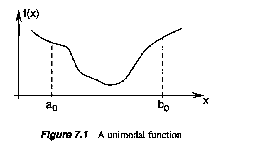
  • The search methods we discuss in this and the next section allow us to determine the minimizer of a function f : R —> R over a closed interval, say [$a_o$, $b_o$]
  • The only property that we assume of the objective function f is that it is unimodal(단 한가지의 모델)
    • which means that f has only one local minimizer
  • The methods we discuss are based on evaluating the objective function at different points in the interval [$a_o$, $b_o$]
  • We choose these points in such a way that an approximation to the minimizer of / may be achieved in as few evaluations as possible.
  • Our goal is to progressively narrow the range until the minimizer is “boxed in” with sufficient accuracy.

  • Consider a unimodal function / of one variable and the interval [$a_o$, $b_o$].
    • If we evaluate / at only one intermediate point of the interval, we cannot narrow the range within which we know the minimizer is located.
    • We have to evaluate f at two intermediate points
    • We choose the intermediate points in such a way that the reduction in the range is symmetric, in the sense that:

  • We then evaluate f at the intermediate points

  • If f($a_1$) < f($a_2$), then the minimizer must lie in the range [$a_0$, $b_1$]. If, on the other hand,f($a_1$) >= f($a_2$), then the minimizer is located in the range [$a_1$, $b_0$]

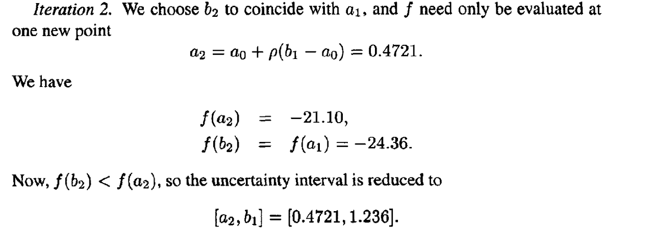
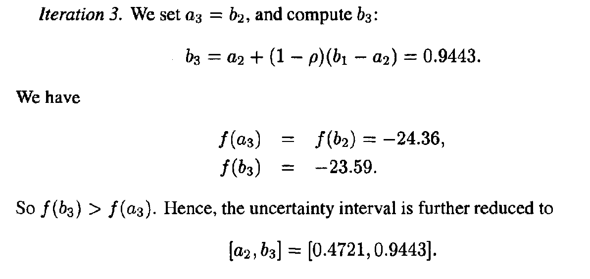
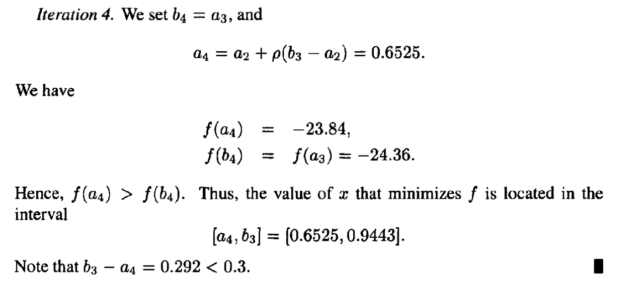
  • Starting with the reduced range of uncertainty we can repeat the process and similarly find two new points, say $a_2$ and $b_2$ using the same value of p < 1/2
  • However, we would like to minimize the number of the objective function evaluations while reducing the width of the uncertainty interval.
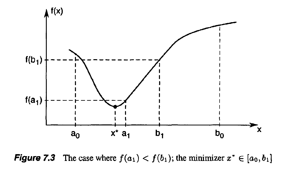
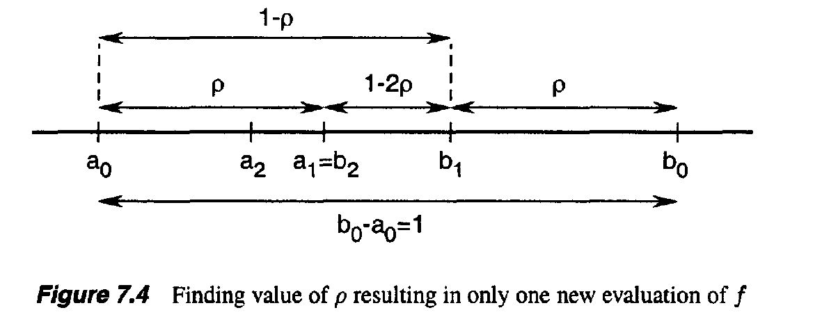
  • Suppose, for example, that f($a_1$) < f($b_1$), as in Figure 7.3.

  • Because $a_1$ is already in the uncertainty interval and f ( $a_1$ ) is already known, we can make $a_1$ coincide with $b_2$
  • Thus, only one new evaluation of f at $a_2$ would be necessary

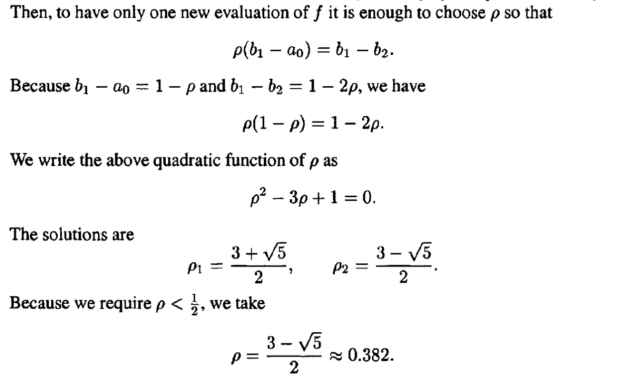
  • To find the value of p that results in only one new evaluation of f
  • Without loss of generality, imagine that the original range [$a_0$, $b_0$] is of unit length.

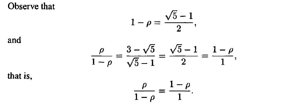
  • Thus, dividing a range in the ratio of p to 1 — p has the effect that the ratio of the shorter segment to the longer equals the ratio of the longer to the sum of the two.
  • This rule was referred to by ancient Greek geometers as the Golden Section.
  • Using this Golden Section rule means that at every stage of the uncertainty range reduction (except the first one), the objective function f need only be evaluated at one new point.
  • The uncertainty range is reduced by the ratio 1 — p = 0.61803 at every stage.
  • Hence, N steps of reduction using the Golden Section method reduces the range by the factor

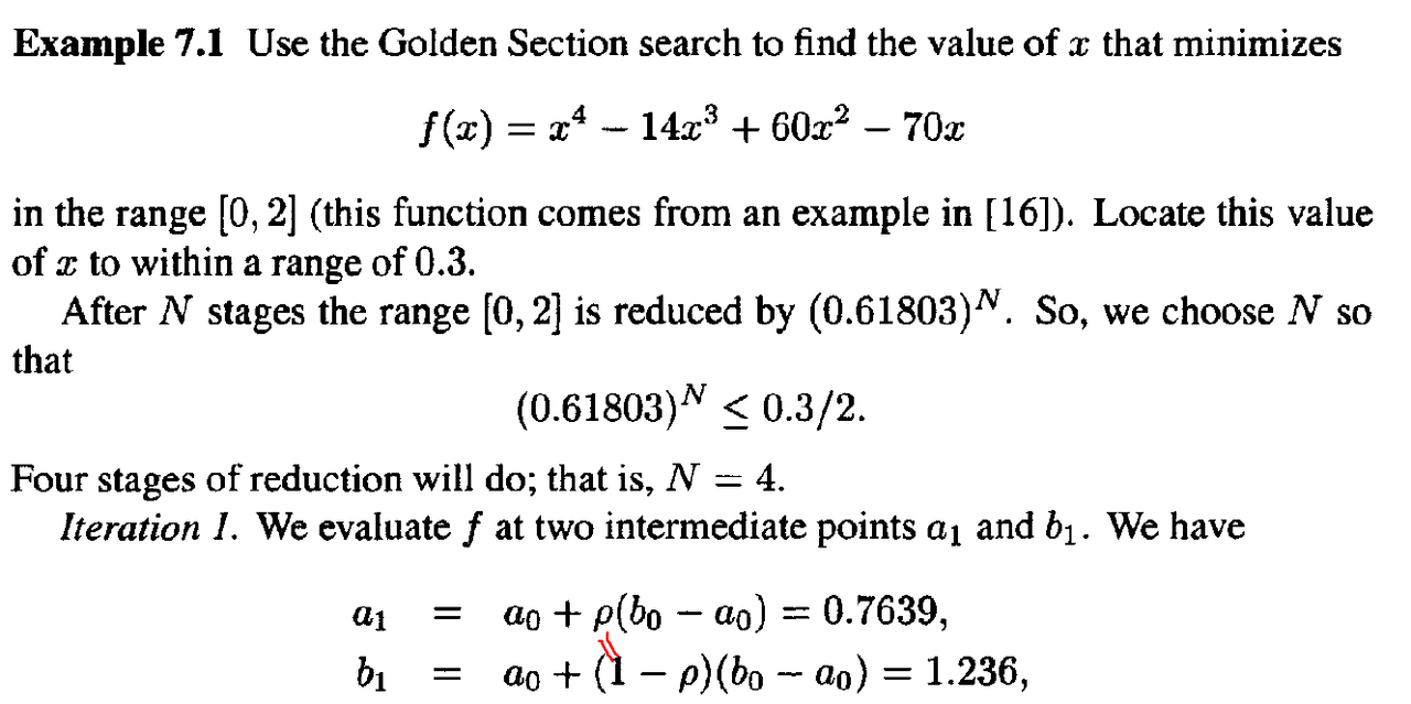
Example

2. FIBONACCI SEARCH

  • Recall that the Golden Section method uses the same value of p throughout
  • Suppose now that we are allowed to vary the value p from stage to stage, so that at the k th stage in the reduction process we use a value $p_k$, at the next stage we use a value p(k+1), and so on.

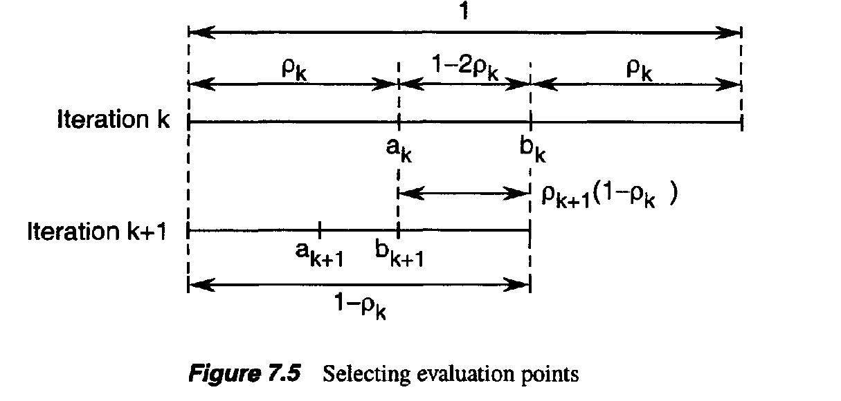
  • As in the Golden Section search, our goal is to select successive values of $p_k$, 0 < $P_k$ < 1/2, such that only one new function evaluation is required at each stage.
  • From Figure 7.5, we see that it is sufficient to choose the $p_k$ such that:

  • There are many sequences $p_1$,$p_2$, • • • that satisfy the above law of formation, and the condition that 0 < $p_k$ < 1/2.

  • Suppose that we are given a sequence $p_1$,$p_2$, - - • satisfying the above conditions, and we use this sequence in our search algorithm.
  • Then, after N iterations of the algorithm, the uncertainty range is reduced by a factor of

  • Depending on the sequence $p_1$,$p_2$,…, we get a different reduction factor.
  • The natural question is as follows: What sequence $p_1$,$p_2$,… minimizes the above reduction factor?
  • This problem is a constrained optimization problem that can be formally stated:

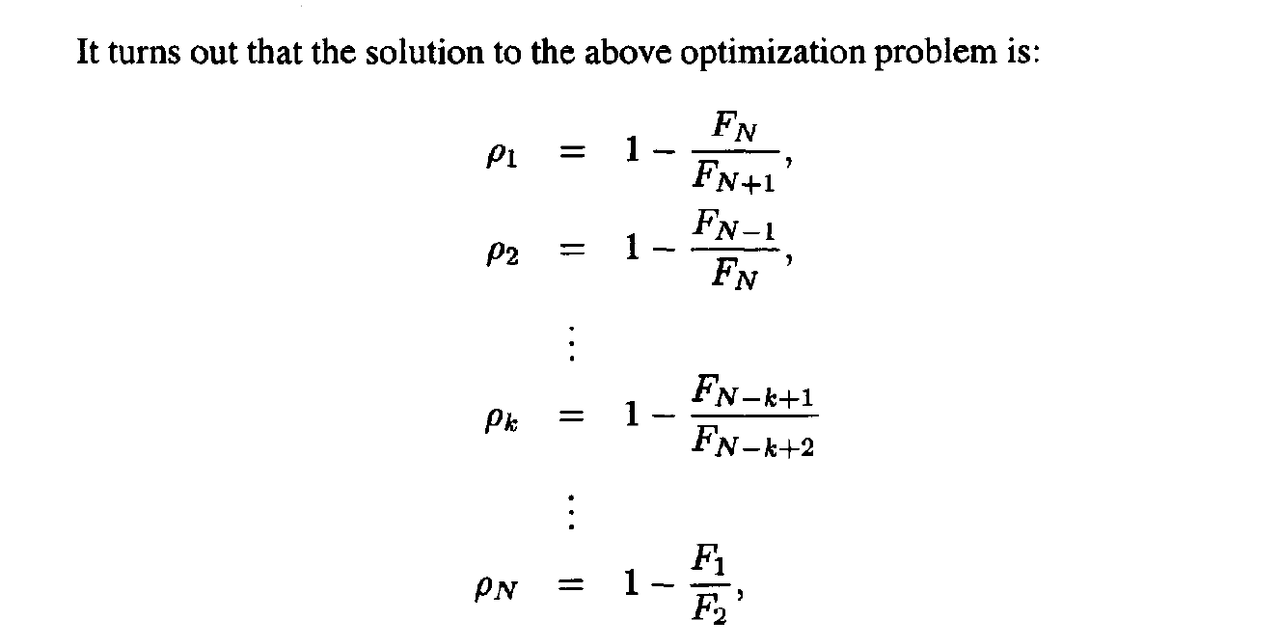
  • Before we give the solution to the above optimization problem, we first need to introduce the Fibonacci sequence, FI,F2,F3, — This sequence is defined as follows. First, let F(-1) = 0 and F(0) = 1 by convention. Then, for k > 0,

  • where the $F_k$ are the elements of the Fibonacci sequence.
  • The resulting algorithm is called the Fibonacci search method.
  • In the Fibonacci search method, the uncertainty range is reduced by the factor:

  • Because the Fibonacci method uses the optimal values of $p_1$,$p_2$, • • •» the above reduction factor is less than that of the Golden Section method.
  • In other words, the Fibonacci method is better than the Golden Section method in that it gives a smaller final uncertainty range.
  • We point out that there is an anomaly in the final iteration of the Fibonacci search method, because:

  • Recall that we need two intermediate points at each stage, one that comes from a previous iteration and another that is a new evaluation point.
  • However, with $p_N$ = 1/2, the two intermediate points coincide in the middle of the uncertainty interval, and therefore we cannot further reduce the uncertainty range.
  • To get around, this problem, we perform the new evaluation for the last iteration using $p_N$ = 1/2 - ε, where ε is the small number
  • In other words, the new evaluation point is just to the left or right of the midpoint of the uncertainty interval.
  • This modification to the Fibonacci method is, of course, of no significant practical consequence
  • As a result of the above modification, the reduction in the uncertainty range at the last iteration may be either

  • depending on which of the two points has the smaller objective function value.
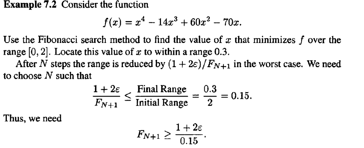
  • Therefore, in the worst case, the reduction factor in the uncertainty range for the Fibonacci method is

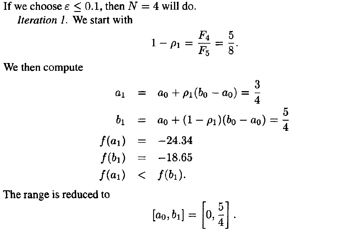
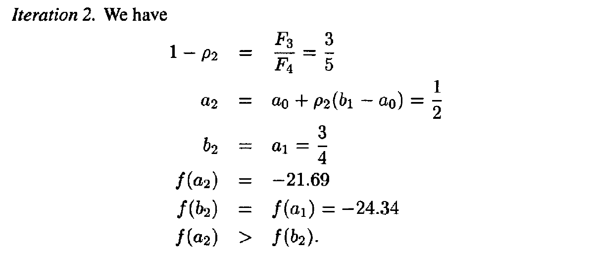
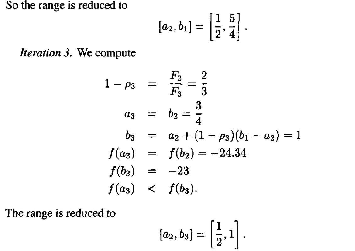
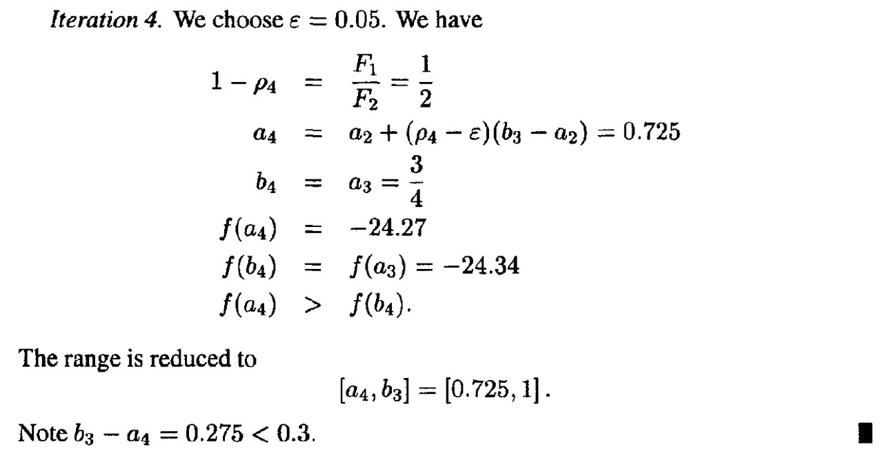
Example

3. NEWTON’S METHOD

  • Suppose again that we are confronted(降临于) with the problem of minimizing a function f of a single real variable x.
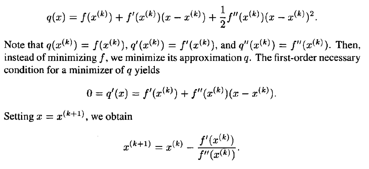
  • We assume now that at each measurement point $x^k$ we can calculate f($x^k$), f’’($x^k$}, and f’’’($x^k$). We can fit a quadratic function through $x^k$ that matches its first and second derivatives with that of the function f.
  • This quadratic has the form :

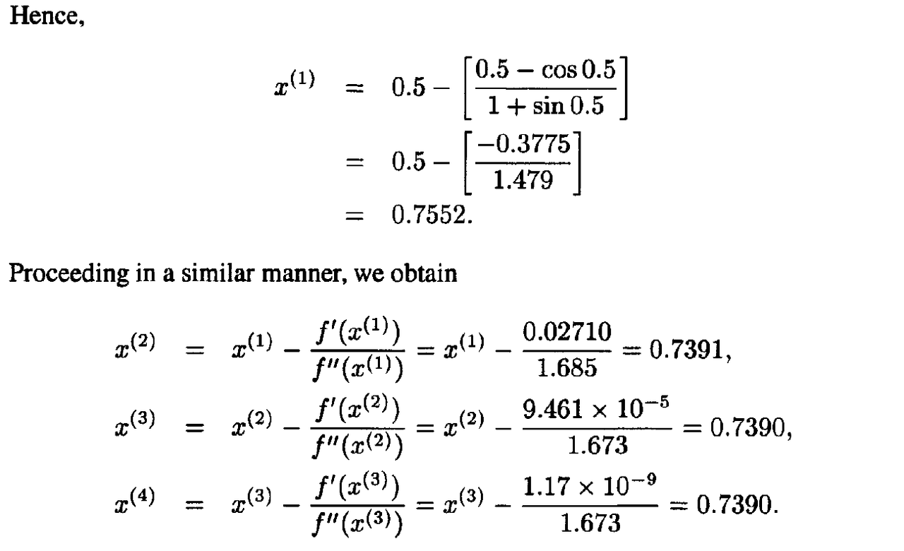
Example 1

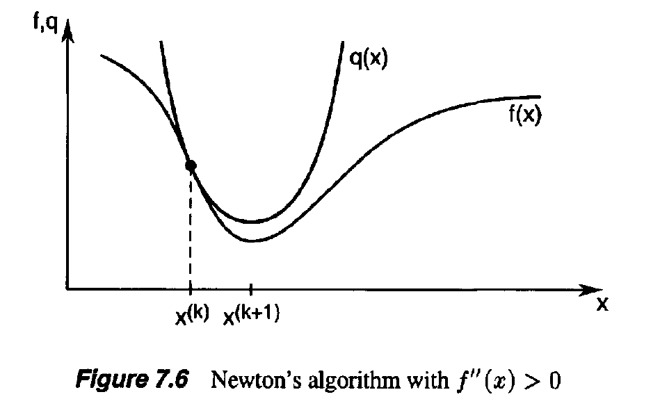
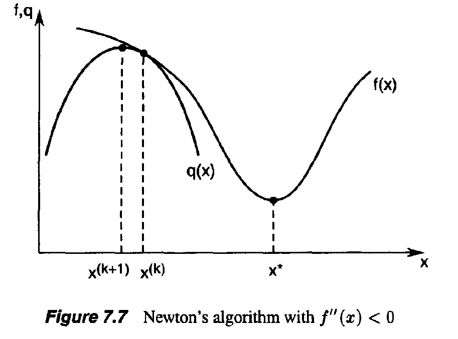
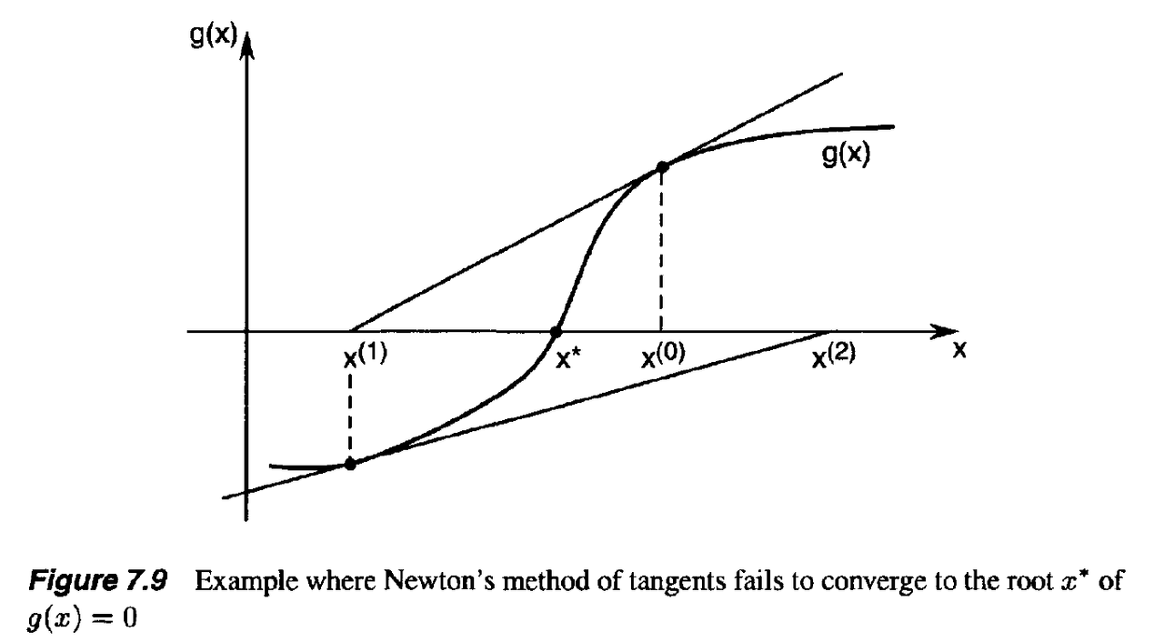
  • Newton’s method works well if f “ ( x ) > 0 every where (see Figure 7.6). However, if f”(x) < 0 for some x, Newton’s method may fail to converge to the minimizer (see Figure 7.7).

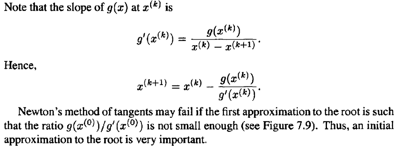
  • Newton’s method can also be viewed as a way to drive the first derivative of f to zero. Indeed, if we set g(x) = f ‘ ( x ) , then we obtain a formula for iterative solution of the equation g(x) = 0:

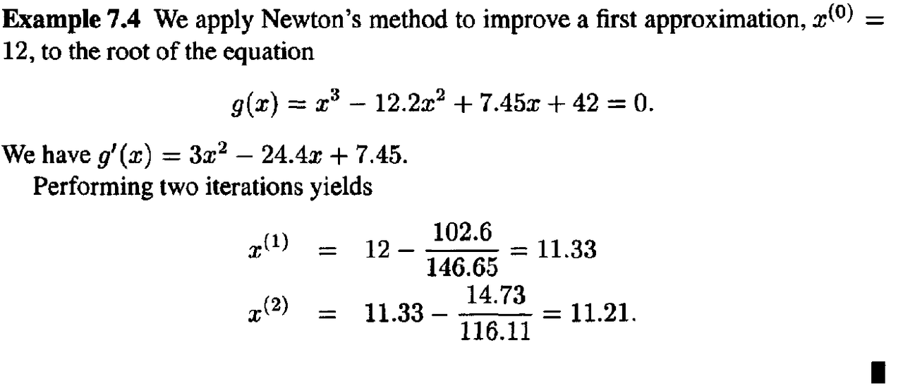
Example 2

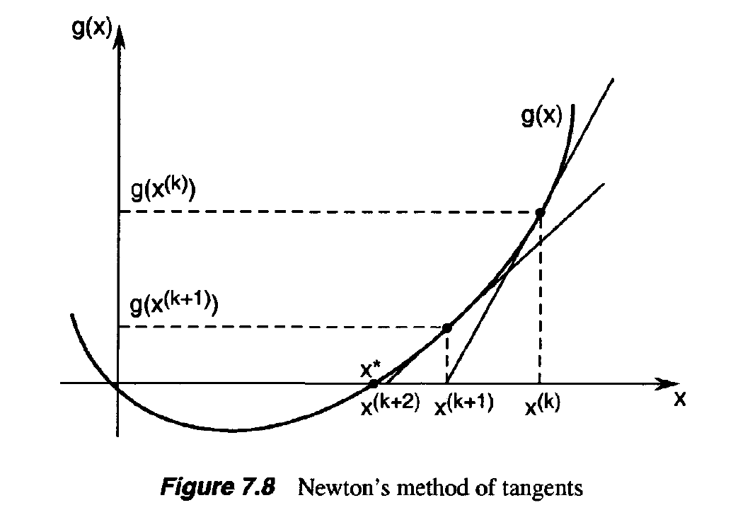
  • Newton’s method for solving equations of the form g(x) = 0 is also referred to as Newton’s method of tangents.
  • This name is easily justified if we look at a geometric interpretation of the method when applied to the solution of the equation g(x) = 0

  • If we draw a tangent to g(x) at the given point $x^k$, then the tangent line intersects the x-axis at the point x^(k+1), which we expect to be closer to the root x* of g(x) = 0.

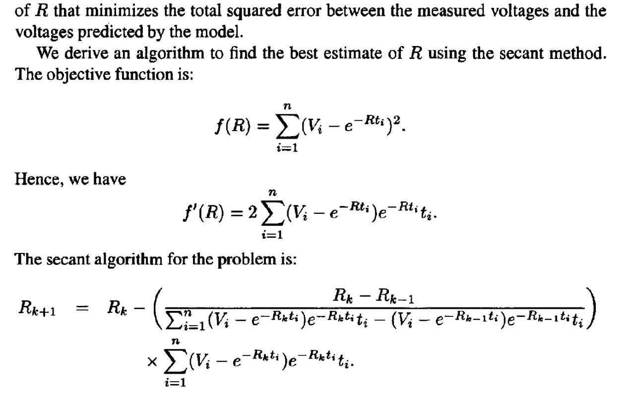
4. SECANT METHOD

  • Newton’s method for minimizing f uses second derivatives of f:

  • If the second derivative is not available, we may attempt to approximate it using first derivative information.
  • In particular, we may approximate f”($x^k$} above with

  • Using the above approximation of the second derivative, we obtain the algorithm:

  • The above algorithm is called the secant method.
  • Note that the algorithm requires two initial points to start it, which we denote x^(-1) and x^(0)
  • The secant algorithm can be represented in the following equivalent form:

  • Observe that, like Newton’s method, the secant method does not directly involve values of f($x^k$). Instead, it tries to drive the derivative f’ to zero.
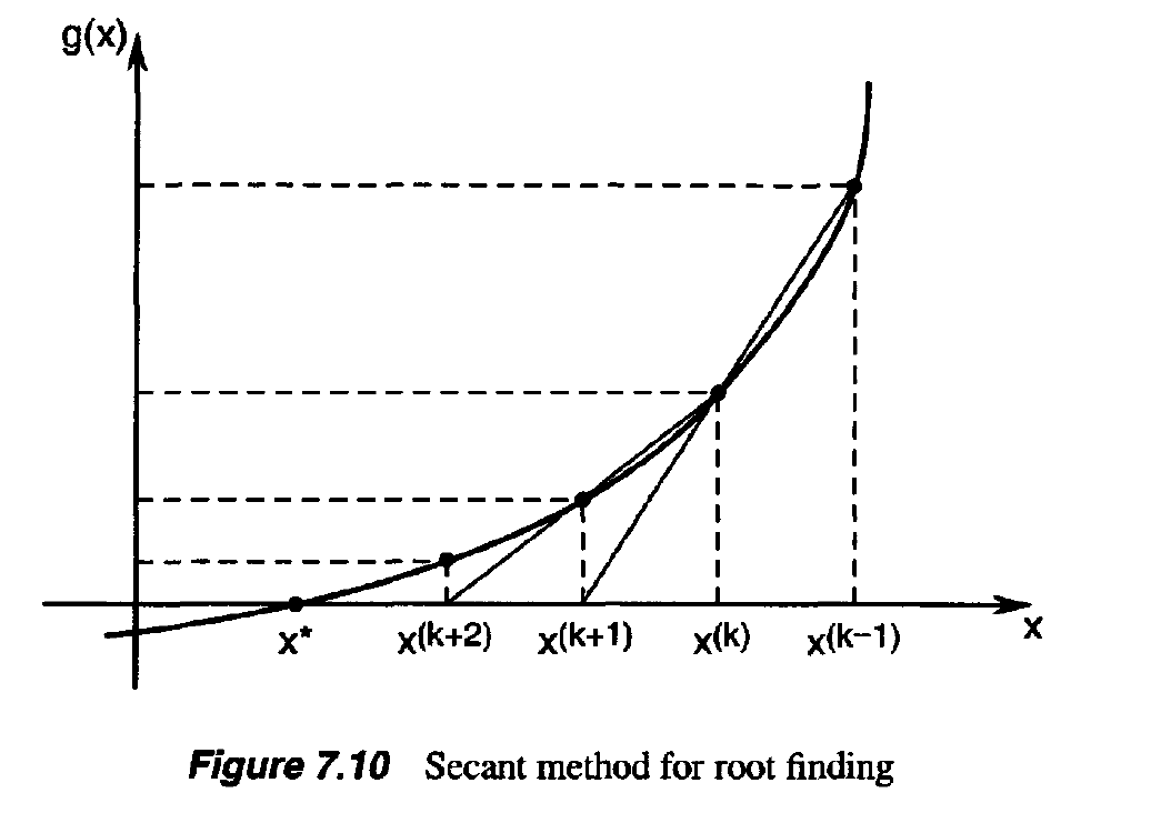
  • In fact, as we did for Newton’s method, we can interpret the secant method as an algorithm for solving equations of the form g(x) =Q.
  • Specifically, the secant algorithm for finding a root of the equation g(x) = 0 takes the form

  • The secant method for root finding is illustrated in Figure 7.10 (compare this with Figure 7.8).
  • Unlike Newton’s method, which uses the slope of g to determine the next point, the secant method uses the “secant” between the (k — l)st and kth points to determine the (k + l)st point.

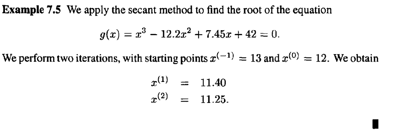
Example 1

Example 2

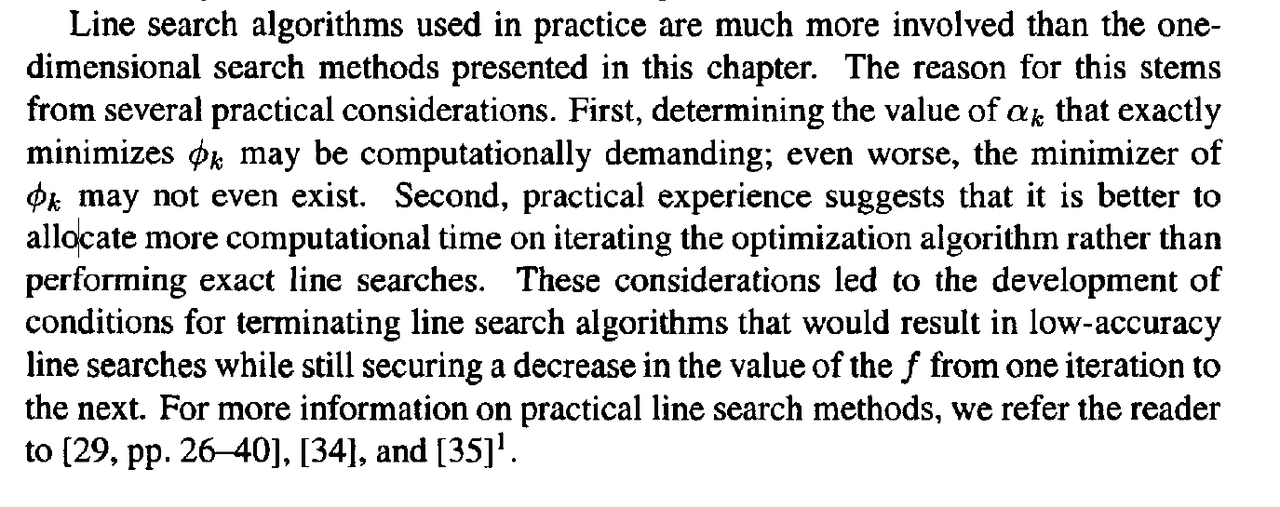
5. REMARKS ON LINE SEARCH METHODS

  • One-dimensional search methods play an important role in multidimensional optimization problems
  • In particular, iterative algorithms for solving such optimization problems (to be discussed in the following chapters) typically involve a “line search” at every iteration.
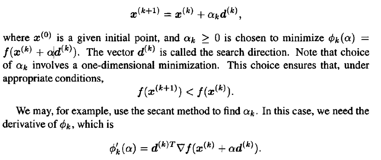
  • To be specific, let / : W1 -4 R be a function that we wish to minimize.
  • Iterative algorithms for finding a minimizer of f are of the form:

  • The above is obtained using the chain rule.
  • Therefore, applying the secant method for the line search requires the gradient f.
  • the initial line search point $x^k$ and the search direction $d^k$
  • Of course, other one-dimensional search methods may be used for line search

Reference

Optimization method - Standford University

https://www.youtube.com/results?search_query=convex+function

Comment  Read more

23. N-step Methods

|

N-step Methods

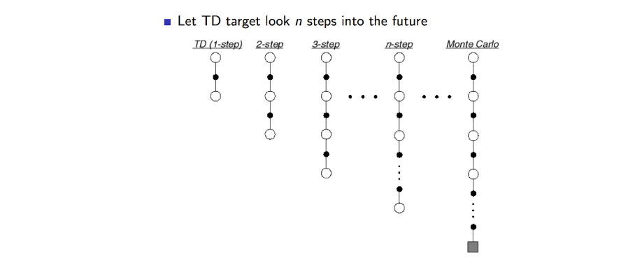
  • N-step Methods : Further our understanding of TD methods
  • we know so far: TD(0)
  • we will learn :
    • λ = 0 gives us TD(0), λ = 1 gives us monte Carlo
  • any other λ is a trade-off(协调) between the two

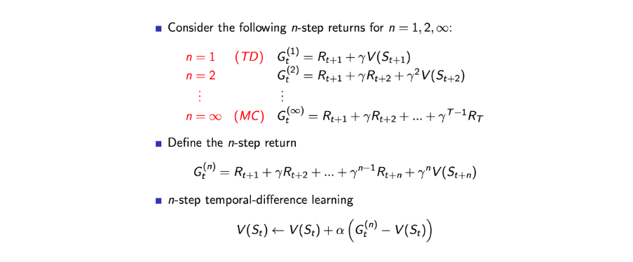
  • 1-Step TD의 step을 증가시켜 나가면서 n까지 보게 된다면 n-step TD로 일반화 할 수 있다.
  • 만약 step이 무한대에 가깝게 되면 MC와 동일하게 될 것이다.
  • 2-Step TD에서 업데이트 방식은 척번째 보상과 두번째 보상 그리고 부전째 상태에서의 Value function의 합으로 업데이트가 된다.

  • n step TD에서의 Value 함수는 N-step 에서 얻은 총 보상에서 기존 Value 함수값과 차이를 알파만큼 가중치하여 더함으로서 업데이트가 되게 됩니다.

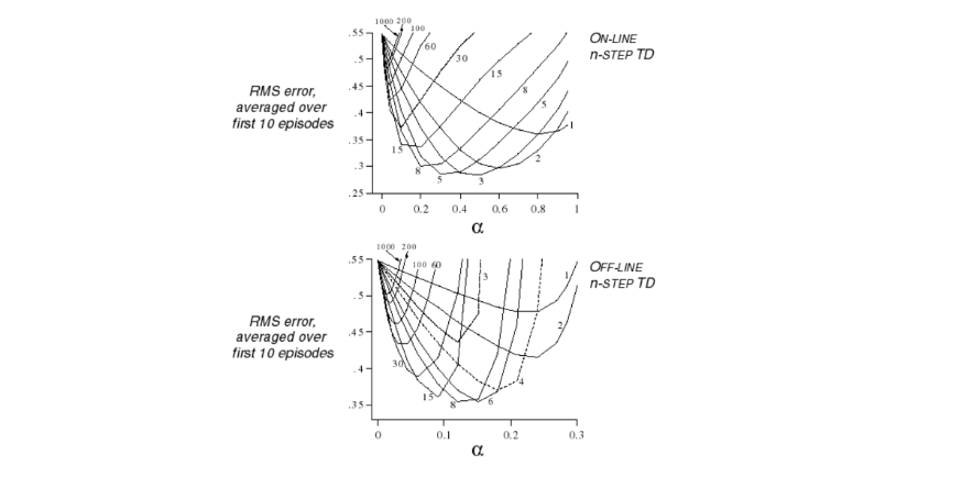
  • n 이 몇일때가 가장 최고의 결과값늘 나타낼까? 위에 그래프가 실험에 대한 결과 값입니다.
  • 실시간 업데이트하는 온라인 방식, 에피소드 완료후 업데이트하는 오프라인 방식에 대한 결과는 비슷하게 나온다.
  • n이 커질수록 에러가 커지는 것을 볼 수 있다.
  • 3~5 step 이 좋은거 같다.

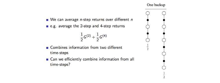
  • n-step 에서 보상값을 다른 값으로 평균을 낼 수 있다.
  • 하지만 2~4 step에서의 평균을 내어보면 위와 같은 식이 될 것이다.
  • 이 두가지를 결합하여 효율적으로 만들수 있을까?

  • 답은 가능하다
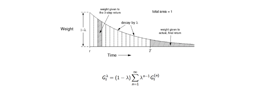
  • 여기서 람다 보상은 모든 n-step 까지의 가중평균된 보상이다.
  • 기존에 n-step에서 사용한 보상은 총합이였다.
  • 이렇게 평균을 이용하는 방식은 오류를 더 낮출 수 있다.
  • 람다의 총합이 1 되도록 하기 위해 (1-lamda)계수로 노멀라이즈를 하여 0부터 1까지의 값을 갖도록 합니다.
  • 람다는 n-step이 커질 수록 보상에 대한 값을 감소시키게 합니다.
  • 마지막에 공식이 TD-Lamda 의 Value 함수입니다.

  • Step 시간이 흐를수록 weight가 지수형태로 감소하는 것을 볼수 있다.
  • 그리고 이들의 총합은 1이 된다.
  • 지수형태의 가중치 를 사용하는 것이 알고리즘 연상에 효율성을 주고 메모리를 덜 사용하게 되는 이점이 있다.

  • Value 함수가 업데이트 하는 과정
  • 동일하게 n-step까지 도닿라고 나서 얻은 보상들을 lamda를 이용하여 보상값을 업데이트 하게 된다.
  • 정방향의 관점에서 보면 이론접이다.
  • 반대방향 관점에서 보면 컴퓨터 적이다.
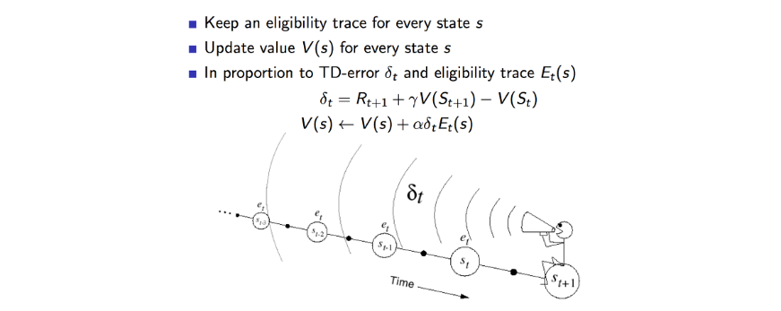
  • 반대 방향으로 보면 TD(Lamda) 알고리즘은 온라인 방식과 같이 매 step마다 업데이트가 된다.

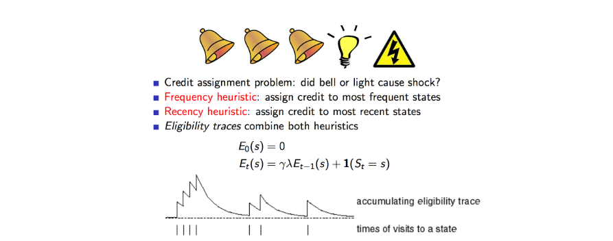
  • 위에서 번개가 발생한 이유는 자주 발생한 것이 영향이 큰지 최근에 발생한 것이 영향이 큰지를 결합하여 사용할 수 있다.
  • 하나의 특정한 state를 방문하는 횟수에 따라서 Eligibility Traces해보면 위에와 같이 나온다.

  • 이를 적용해보면 각 state 마다 업데이트가 발생 될때 TD에러의 비율 만큼 업데이트를 가중적용하는 한다.
  • 이것은 에피소드의 길이보다 짧은 기억을 하는 단기 메모리 같은 역할을 한다.

  • lamda는 얼마나 빨리 값을 감소시키는가를 의미한다.
  • lamda의 값이 0이 되면 완전 가파르게 decay가 발생할 것이다.
  • 결국 현재 state의 value 함수만 업데이트가 되며 니는 TD(0)가 동일한 방식이 된다.

  • 반대로 lamda가 1이 되면 에피소드를 모두 커버하게 된다.
  • MC와 같은 방식으로 오프라인 업데이트가 된다.

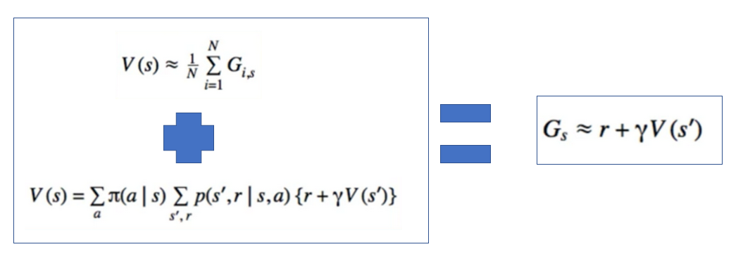
  • value function can be described recursively(bellman’s equation)

  • we can estimate V by taking the sample mean of G’s

  • TD(0) is to combine these 2 things to estimate G itself(all we know for sure is r)

  • All we know for sure is R
  • it’s plausible(有道理的) to ask: what if we use more r’s and less of V?

  • Monte Carlo is just the extreme of this, where we don’t use V at all

  • Let’s superscript G to tell us how many R’s we are using

  • gives us a discrete transition from TD(0) to Monte Carlo
  • TD(0) - wait 1 step to update V
  • Monte Carlo - Wait until end of episode to update V
  • N-step -wait N step to update V
    • why? we need to collect all the R’s

  • For the actual update(which is in terms of G already). no change is needed
  • the only change is to G itself

Control

  • Use Q instead of V
  • Ex. SARSA

Code

# https://deeplearningcourses.com/c/deep-reinforcement-learning-in-python
# https://www.udemy.com/deep-reinforcement-learning-in-python
from __future__ import print_function, division
from builtins import range
# Note: you may need to update your version of future
# sudo pip install -U future
#
# Note: gym changed from version 0.7.3 to 0.8.0
# MountainCar episode length is capped at 200 in later versions.
# This means your agent can't learn as much in the earlier episodes
# since they are no longer as long.   
#
# Adapt Q-Learning script to use N-step method instead

import gym
import os
import sys
import numpy as np
import matplotlib.pyplot as plt
from gym import wrappers
from datetime import datetime

# code we already wrote
import q_learning
from q_learning import plot_cost_to_go, FeatureTransformer, Model, plot_running_avg

SGDRegressor

class SGDRegressor:
  def __init__(self, **kwargs):
    self.w = None
    self.lr = 1e-2

  def partial_fit(self, X, Y):
    if self.w is None:
      D = X.shape[1]
      self.w = np.random.randn(D) / np.sqrt(D)
    self.w += self.lr*(Y - X.dot(self.w)).dot(X)

  def predict(self, X):
    return X.dot(self.w)
    # replace SKLearn Regressor
q_learning.SGDRegressor = SGDRegressor

# calculate everything up to max[Q(s,a)]
# Ex.
# R(t) + gamma*R(t+1) + ... + (gamma^(n-1))*R(t+n-1) + (gamma^n)*max[Q(s(t+n), a(t+n))]
# def calculate_return_before_prediction(rewards, gamma):
#   ret = 0
#   for r in reversed(rewards[1:]):
#     ret += r + gamma*ret
#   ret += rewards[0]
#   return ret

play

# returns a list of states_and_rewards, and the total reward
def play_one(model, eps, gamma, n=5):
    # n is n-step
  observation = env.reset()
  done = False
  totalreward = 0
  rewards = []
  states = []
  actions = []
  iters = 0
  # array of [gamma^0, gamma^1, ..., gamma^(n-1)]
  multiplier = np.array([gamma]*n)**np.arange(n)
  # while not done and iters < 200:
  while not done and iters < 10000:
    # in earlier versions of gym, episode doesn't automatically
    # end when you hit 200 steps
    action = model.sample_action(observation, eps)

    states.append(observation)
    actions.append(action)

    prev_observation = observation
    observation, reward, done, info = env.step(action)

    rewards.append(reward)

    # update the model
    if len(rewards) >= n:
      # return_up_to_prediction = calculate_return_before_prediction(rewards, gamma)
      return_up_to_prediction = multiplier.dot(rewards[-n:])
      G = return_up_to_prediction + (gamma**n)*np.max(model.predict(observation)[0])
      model.update(states[-n], actions[-n], G)

    # if len(rewards) > n:
    #   rewards.pop(0)
    #   states.pop(0)
    #   actions.pop(0)
    # assert(len(rewards) <= n)

    totalreward += reward
    iters += 1

  # empty the cache
  if n == 1:
    rewards = []
    states = []
    actions = []
  else:
    rewards = rewards[-n+1:]
    states = states[-n+1:]
    actions = actions[-n+1:]
  # unfortunately, new version of gym cuts you off at 200 steps
  # even if you haven't reached the goal.
  # it's not good to do this UNLESS you've reached the goal.
  # we are "really done" if position >= 0.5
  if observation[0] >= 0.5:
    # we actually made it to the goal
    # print("made it!")
    while len(rewards) > 0:
      G = multiplier[:len(rewards)].dot(rewards)
      model.update(states[0], actions[0], G)
      rewards.pop(0)
      states.pop(0)
      actions.pop(0)
  else:
    # we did not make it to the goal
    # print("didn't make it...")
    while len(rewards) > 0:
      guess_rewards = rewards + [-1]*(n - len(rewards))
      G = multiplier.dot(guess_rewards)
      model.update(states[0], actions[0], G)
      rewards.pop(0)
      states.pop(0)
      actions.pop(0)

  return totalreward

main

if __name__ == '__main__':
  env = gym.make('MountainCar-v0')
  ft = FeatureTransformer(env)
  model = Model(env, ft, "constant")
  gamma = 0.99

  if 'monitor' in sys.argv:
    filename = os.path.basename(__file__).split('.')[0]
    monitor_dir = './' + filename + '_' + str(datetime.now())
    env = wrappers.Monitor(env, monitor_dir)


  N = 300
  totalrewards = np.empty(N)
  costs = np.empty(N)
  for n in range(N):
    # eps = 1.0/(0.1*n+1)
    eps = 0.1*(0.97**n)
    totalreward = play_one(model, eps, gamma)
    totalrewards[n] = totalreward
    print("episode:", n, "total reward:", totalreward)
  print("avg reward for last 100 episodes:", totalrewards[-100:].mean())
  print("total steps:", -totalrewards.sum())

  plt.plot(totalrewards)
  plt.title("Rewards")
  plt.show()

  plot_running_avg(totalrewards)

  # plot the optimal state-value function
  plot_cost_to_go(env, model)

Reference:

Artificial Intelligence Reinforcement Learning

Advance AI : Deep-Reinforcement Learning

Cutting-Edge Deep-Reinforcement Learning

Comment  Read more