for Robot Artificial Inteligence

11. Introduction to Dynamic Programming

|

intro to Dynamic Programming

  • Solutions to MDPs
  • Centrepiece of MDP: The bellman Equation
  • if we look carefully, this can be used to solve for V(s) Directly
  • I S I equations, I S I unknowns(linear Problem)
  • Many entries(进入(指行动)) will be 0, since transitions s -> s’ are sparse
  • Instead, we will use Iterative Policy evaluation

1. Iterative Policy evaluation

def iterative_policy_evaluation(π):
  initialize V(s) = 0 for all s ∈ S
  while true :
    ∆ = 0
    for each s ∈ S:
      old_v = V(s)

     ∆ = max(∆, I V(s) - old_v I )
     if ∆ < Threshold: break

     return V(s)
  • Technically, it’s defined where V(s) at iteration k+1 is updated from V(s) at iteration k
  • But we can update V(s) “in place”, to use the most recently updated values
  • Converges(汇集) Faster

Definition

  • What we just did(Finding V(s) given a policy) is called the Prediction Problem
  • Finding the optimal policy is called the Control Problem

2. Designing our RL Program

  • Let’s recap how to do this in supervised learning
class MyModel;
  def fit(x,y):
    # our job
  def predict(x)
    # our job
# boilerplate
Xtrain, Ytrain, Xtest, Ytest = get_data() # 1. Get Data
Model = MyModel() # 2. Instantiate Model
model.fit(Xtrain,Ytrain) # 3. Train Model
model.score(Xtest, ytest) # 4. Evaluation Model
  • RL Program is not supervised learning but there is still a pattern to be followed
  • Same as bandit section: several algorithms, but all have the same interface
  • Only the algorithm is different, not the layout
  • Applies to all the RL algorithms
  • Designing our RL Program, there are t types of problems
    1. Prediction Problem: Given a policy, find V(s)
    • Goal: Find V(s)
      given: policy
      V(s) = initial value
      for t in range(max_iterations):
      states, actions, rewards = play_game(policy)
      update V(s) given (state, actions, rewards)
      print useful info (change in V(s) vs time, final V(s), policy)
      
      2. Control Problem : Find the optimal policy and the corresponding value function
      
    • Goal : find the optimal Policy
    • note : Policy may not be explicitly represented
      initialize value function and Policy
      for t in range(max_iterations):
      states, actions, rewards = play_game(policy)
      update Value function and policy to (states, actions,rewards) using the algorithm
      print useful info (change in V(s) vs time, final V(s), final policy)
      

3. Iterative Policy Evaluation

  • we will look at 2 different Policies
  • First: Completely random(Uniform) policy
  • which is relavant?
    • π(a I s)
    • p(s’,r I s,a)
  • Answer : π(a I s)
  • for a uniformly random policy, this will be 1/IA(s)I
  • A(s) = set of possible actions from state s
  • p(s’,r I s,a) is only relevant when state transitions are random

  • Second: policy we we’ll look at is Completely deterministic
  • from start position, we go Directly to goal
  • otherwise, we go Directly to losing state

4. Policy Improvement

  • THe control Problem
  • How to find better policies -> optimal policy
  • what we know so far : how to find V/Q given a fixed policy
  • using the current policy, we simply get the state-value function
  • can we change just this one action for s? i.e. choose a != π(s)
  • Yes
  • we have a finite set of actions, so just go through each one until we get a better Q
  • this looks complicated, but it’s very simple
  • all it’s saying is, if the policy for state s is to currently go “up”
  • just check “left”, “right”, and “down” to see if we can get a bigger Q
  • if so, change our policy for state s to the new action
  • Formally, we’re finding a new policy π’, that gives us a givver value than we had before:
  • if we have Q:
  • if we have V:
  • Notice : it’s greedy
  • we never consider globally the value function at all states
  • only look at current state s
  • notice: it uses an imperfect version of $V_π$(s)
  • once we change π. $V_π$(s) also changes
  • when are we finished changing the policy, it doesn’t change when we try policy Improvement, V(s) also doesn’t change
  • ”<” when still improving = when finished
  • if we found optimal policy, Value function is always same in state

5. Policy Iteration

  • this is what use to find the optimal policy
  • problem we encountered last lecture: when we change the policy, the value function becomes out of date
  • How do we fix the out-of-date value function?
  • simply recalculate it given the new policy
  • we already know how to find V given π:
    • iterative policy Evaluation
  • High-level: alternate between policy evaluation and policy improvement
  • keep doing this until policy doesn’t change
  • Don’t need to check value function for convergence, because once policy becomes constant so will value

Step of Policy Iteration

  1. Randomly initialize V(s) and the policy π(s)
  2. V(s) = iterative_policy_evaluation(π)
  3. algorithm
policy_changed = False
for s in all_state:
  old_a = policy(s)
  policy(s) = argmax[a]{sum[s',r]{p(s',r I s, a )[ r+ gamma*V(s')]}}
  if policy(s) != old_a: policy_changed = true
if policy_changed: go back to step 2

6. Example (Windy Gridworld)

  • recall, we have 2 probability distributions to deal with:
    • π(a I s)
    • p(s’,r I s,a)
  • so far, p(s’,r I s,a) has been deterministic
  • in windy Gridworld, it’s not
  • imagine we are walking on a windy street. we try to walk straight but wind push we back or left.
  • same thins in windy Gridworld
  • if agent tries to go “up”, it will do so with probability 0.5
  • But it can also go “left”, “down”, or “right” with probability 0.5/3

code

# https://deeplearningcourses.com/c/artificial-intelligence-reinforcement-learning-in-python
# https://www.udemy.com/artificial-intelligence-reinforcement-learning-in-python
from __future__ import print_function, division
from builtins import range
# Note: you may need to update your version of future
# sudo pip install -U future


import numpy as np
from grid_world import standard_grid, negative_grid
from iterative_policy_evaluation import print_values, print_policy

SMALL_ENOUGH = 1e-3
GAMMA = 0.9
ALL_POSSIBLE_ACTIONS = ('U', 'D', 'L', 'R')

# next state and reward will now have some randomness
# you'll go in your desired direction with probability 0.5
# you'll go in a random direction a' != a with probability 0.5/3

if __name__ == '__main__':
  # this grid gives you a reward of -0.1 for every non-terminal state
  # we want to see if this will encourage finding a shorter path to the goal
  grid = negative_grid(step_cost=-1.0)
# what is the step_cost? for example, if we are three steps away from the goal
# we get minus three reward before we even have a chance to get to the goal
# if we are only one step away from the losing state, then we only get minus one reward
  # grid = negative_grid(step_cost=-0.1)
  # grid = standard_grid()

  # print rewards
  print("rewards:")
  print_values(grid.rewards, grid)

  # state -> action
  # we'll randomly choose an action and update as we learn
  policy = {}
  for s in grid.actions.keys():
    policy[s] = np.random.choice(ALL_POSSIBLE_ACTIONS)

  # initial policy
  print("initial policy:")
  print_policy(policy, grid)

  # initialize V(s)
  V = {}
  states = grid.all_states()
  for s in states:
    # V[s] = 0
    if s in grid.actions:
      V[s] = np.random.random()
    else:
      # terminal state
      V[s] = 0

  # repeat until convergence - will break out when policy does not change
  while True:

    # policy evaluation step - we already know how to do this!
    while True:
      biggest_change = 0
      for s in states:
        old_v = V[s]
#         print(old_v)

        # V(s) only has value if it's not a terminal state
        new_v = 0
        if s in policy:
          for a in ALL_POSSIBLE_ACTIONS:
            if a == policy[s]:
              p = 0.5
            else:
              p = 0.5/3
            grid.set_state(s)
            r = grid.move(a)
            new_v += p*(r + GAMMA * V[grid.current_state()])
          V[s] = new_v
          biggest_change = max(biggest_change, np.abs(old_v - V[s]))

      if biggest_change < SMALL_ENOUGH:
        break

    # policy improvement step
    is_policy_converged = True
    for s in states:
      if s in policy:
        old_a = policy[s]
        new_a = None
        best_value = float('-inf')
        # loop through all possible actions to find the best current action
        for a in ALL_POSSIBLE_ACTIONS: # chosen action
          v = 0
          for a2 in ALL_POSSIBLE_ACTIONS: # resulting action
            if a == a2:
              p = 0.5
            else:
              p = 0.5/3
            grid.set_state(s)
            r = grid.move(a2)
            v += p*(r + GAMMA * V[grid.current_state()])
          if v > best_value:
            best_value = v
            new_a = a
        policy[s] = new_a
        if new_a != old_a:
          is_policy_converged = False

    if is_policy_converged:
      break

  print("values:")
  print_values(V, grid)
  print("policy:")
  print_policy(policy, grid)
  # result: every move is as bad as losing, so lose as quickly as possible

6. Value Iteration

  • Alternative technique for solving the control Problem called value iteration
  • Previous technique: policy Iteration
  • Disadvantage of policy iteration:
    • iterative algorithm
      • inside another iterative algorithm
  • Value Iteration is that Policy evaluation step ends when V coverages
  • is there a point before V Converges, s.t the resulting greedy policy wouldn’t change?
  • Yes
  • therefore, we don’t need to wait for policy evaluation to finish. just do a few steps
  • because the policy improvement step will find the same policy anyway
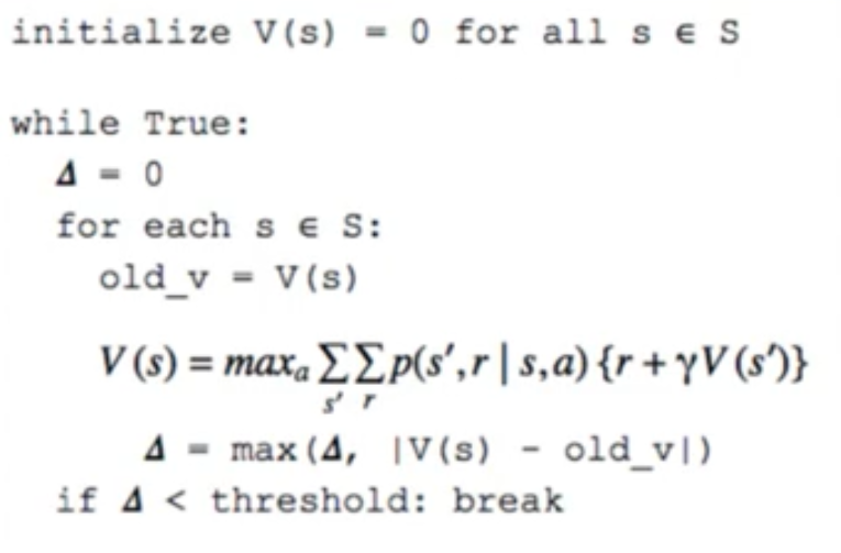
  • Value iteration takes this one step further
  • it combines policy evaluation and policy improvement into one step:
  • what is the difference? taking the max over all possible action
  • Iterative, but don’t need to wait for (k)th iteration of V finish before calculating (k+1)th
  • just update it “in-place(在正确的位置)” as before
  • since policy improvement uses argmax, by taking the max, we’re just doing the next policy evaluation step without calculating policy explicitly

7. Summary

  • Last section : Defined Markov Decision Process
  • This section : one method for finding solutions to MDP: Dynamic Programming
  • Prediction Problem: Iterative Policy evaluation
  • Control Problem: Policy iteration, Value iteration
    • finding the optimal policy and optimal value function

Asynchronous(不同时存在) Dynamic Programming

  • Every DP algorithm we looked at involved looping through entire set of states
  • Recall that for many realistic games, state space is ridiculously large
  • thus, even one iteration can take a long time
  • one way to speed up: update V(s) “in-place”
  • we can take that one step further: Asynchronous(不同时存在) Dynamic Programming
  • instead of looping through all states, loop through a few or only one
  • Choose based one which states are most-visited
    • can be learned by playing the game

Generalized Policy iteration

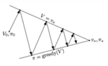
  • Main concept behind policy iteration: we iteratively alternate between 2 steps - policy evaluation and policy improvement
  • Converge when bellman’s equation becomes true(i.e. V(s) = right-hand side)
Efficiency of DP

  • Consider how long it would take to do brute force search
  • . # States = N, # actions = M
  • if we assume we can go from start to goal state in O(N) time, then we want to explore action sequences of length O(N)
  • M x M x … x M
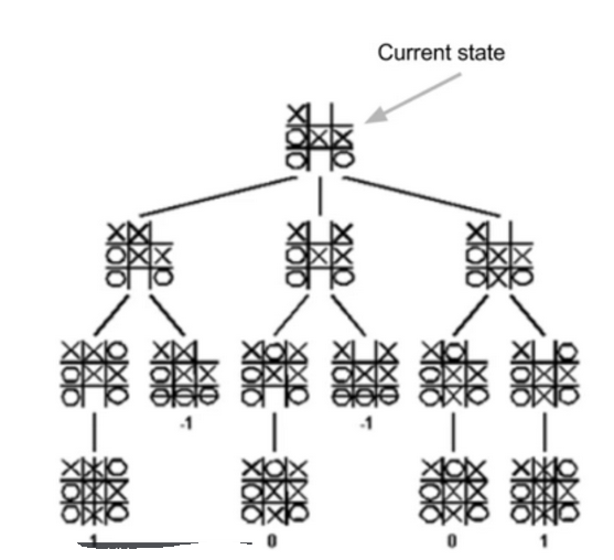
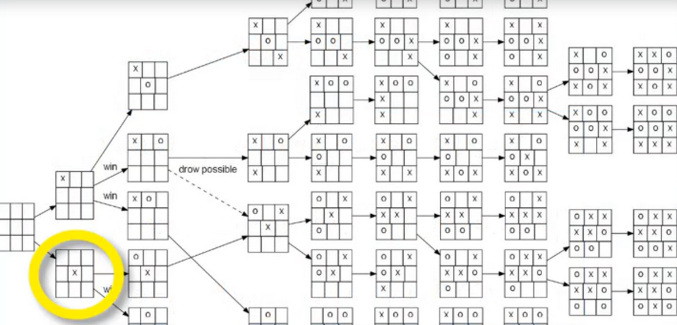
  • we did this problem earlier in tic-tac-toe section
  • of possible permutation(排列(方式)) is O(M^n)

  • Once we generate all possible sequences, do policy evaluation on all to find the best V(s)
  • exponential in # of states

Model-based vs Model-free

  • Notice how DP requires full model of the environment
  • In Particular, p(s’,r I s,a)
  • In the real world, these may be hard to measuring, especially if ISI is large
  • next sections will look at methods which don’t require such a model - called model-free methods
  • also notice there iterative methods requires an initial estimate
  • we make estimates from other estimates (V(s) and policy )
  • Making an initial estimate is called Bootstrapping
  • Monte Carlo (MC) Does not require boot Bootstrapping
  • Temporal difference(TD) learning does

Reference:

Artificial Intelligence Reinforcement Learning

Advance AI : Deep-Reinforcement Learning

Cutting-Edge Deep-Reinforcement Learning

Comment  Read more

29. Standard Template library(STL) - Vector

|

Standard Template Library (STL)

  • C++ 표준 라이브러리를 보면 꽤나 많은 종류의 라이브러리들이 있습니다.
  • 대표적으로 입출력 라이브러리 (iostream 등등), 시간 관련 라이브러리 (chrono), 정규표현식 라이브러리 (regex) 등등 들이 있지요.
  • 하지만 보통 C++ 템플릿 라이브러리(STL)를 일컫는다면 다음과 같은 세 개의 라이브러리들을 의미합니다
    • 임의 타입의 객체를 보관할 수 있는 컨테이너 (container)
    • 컨테이너에 보관된 원소에 접근할 수 있는 반복자 (iterator)
    • 반복자들을 가지고 일련의 작업을 수행하는 알고리즘 (algorithm)
  • EX
    • 편지를 보관하는 각각의 편지함들은 ‘컨테이너’
    • 편지를 보고 원하는 편지함을 찾는 일은 ‘반복자’
    • 편지들을 편지함에 날짜 순서로 정렬하여 넣는 일은 ‘알고리즘’
  • 임의 타입의 객체를 보관할 수 있는 컨테이너 (container)
    • 우리가 다루려는 객체가 어떤 특성을 갖는지 무관하게 라이브러리를 자유롭게 사용할 수 있다는 것입니다 (because of Template).
    • 만일 사용하려는 자료형이 int 나 string 과 같은 평범한 애들이 아니라, 우리가 만든 임의이 클래스의 객체들이여도 자유롭게 위 라이브러리의 기능들을 모두 활용할 수 있습니다.
  • 반복자의 도입으로 알고리즘 라이브러리에 필요한 최소한의 코드만을 작성할 수 있게 되었습니다.
    • 존의 경우 M 개 종류의 컨테이가 있고 N 종류의 알고리즘이 있다면 이 모든 것을 지원하려면 MN 개의 알고리즘 코드가 있어야만 했습니다.
    • 반복자를 이용해서 컨테이너를 추상화 시켜서 접근할 수 있기 때문에 N 개의 알고리즘 코드 만으로 M 종류의 컨테이너들을 모두 지원할 수 있게됩니다.

STL 컨테이너 - Vector(STD::vector)

  • C++ STL 에서 컨테이너는 크게 두 가지 종류가 있습니다.
    • 먼저 배열 처럼 객체들을 순차적으로 보관하는 시퀀스 컨테이너 (sequence container)
    • 키를 바탕으로 대응되는 값을 찾아주는 연관 컨테이너 (associative container) 가 있습니다.
  • 시퀀스 컨테이너의 경우 vector, list, deque 이렇게 3 개가 정의되어 있습니다.
    • (vector) 의 경우, 쉽게 생각하면 가변길이 배열이
    • 벡터에는 원소들이 메모리 상에서 실제로 순차적으로 저장되어 있고, 따라서 임의의 위치에 있는 원소를 접근하는 것을 매우 빠르게 수행할 수 있습니다.
  • vector 의 경우, 임의의 위치에 있는 원소에 접근을 O(1) 로 수행할 수 있습니다. 게다가 맨 뒤에 새로운 원소를 추가하거나 제거하는 것 역시 O(1) 에 수행합니다.
  • vector 의 임의의 원소에 접근하는 것은 배열처럼 [] 를 이용하거나, at 함수를 이용하면 됩니다.
  • 또한 맨 뒤에 원소를 추가하거나 제거하기 위해서는 push_back 혹은 pop_back 함수를 사용하면 됩니다. 아래 예를 보겠습니다
#include <iostream>
#include <vector>

int main() {
  std::vector<int> vec;
  vec.push_back(10);  // 맨 뒤에 10 추가
  vec.push_back(20);  // 맨 뒤에 20 추가
  vec.push_back(30);  // 맨 뒤에 30 추가
  vec.push_back(40);  // 맨 뒤에 40 추가

  for (std::vector<int>::size_type i = 0; i < vec.size(); i++) {
    std::cout << "vec 의 " << i + 1 << " 번째 원소 :: " << vec[i] << std::endl;
  }
}
  • 벡터의 크기를 리턴하는 함수인 size 의 경우, 그리턴하는 값의 타입은 size_type 멤버 타입으로 정의되어 있습니다.
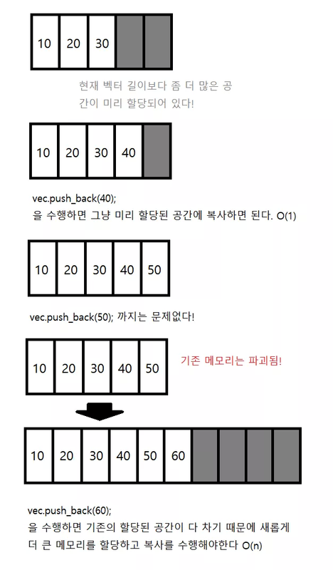
  • 맨 뒤에 원소를 추가하는 작업은 엄밀히 말하자면 amortized O(1) 이라고 합니다. (amortized 의 뜻은 분할상환이란 뜻)
  • 왜냐면 보통은 vector 의 경우 현재 가지고 있는 원소의 개수 보다 더 많은 공간을 할당해 놓고 있습니다.
  • 예를 들어 현재 vector 에 있는 원소의 개수가 10 개라면 이미 20개를 저장할 수 있는 공간을 미리 할당해놓게됩니다.
  • 따라서 만약에 뒤에 새로운 원소를 추가하게 된다면 새롭게 메모리를 할당할 필요가 없이, 그냥 이미 할당된 공간에 그 원소를 쓰기만 하면 됩니다.
  • 따라서 대부분의 경우 O(1) 으로 vector 맨 뒤에 새로운 원소를 추가하거나 지울 수 있습니다.
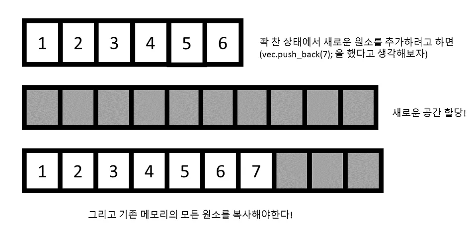
  • 문제가 되는 상황은 할당된 공간을 다 채웠을 때 입니다.
  • 이 때는 어쩔 수 없이, 새로운 큰 공간을 다시 할당하고, 기존의 원소들을 복사하는 수 밖에 없습니다.
  • 따라서 이 경우 n 개의 원소를 모두 복사해야 하기 때문에 O(n) 으로 수행됩니다.
  • 하지만 이 O(n) 으로 수행되는 경우가 매우 드물기 때문에, 전체적으로 평균을 내보았을 때 O(1) 으로 수행됨을 알 수 있습니다.
  • 이렇기에 amortized O(1)O(1) 이라고 부르게 됩니다.

  • vector 기능은 맨 뒤에 원소를 추가하거나 제거하는 것은 빠르지만,임의의 위치에 원소를 추가하거나 제거하는 것은 O(n) 으로 느립니다.
  • 왜냐하면 어떤 자리에 새로운 원소를 추가하거나 뺄 경우 그 뒤에 오는 원소들을 한 칸 씩 이동시켜 주어야만 하기 때문이지요. 따라서 이는 nn 번의 복사가 필요로 합니다.
  • 따라서 만일 맨 뒤가 아닌 위치에 데이터를 추가하거나 제거하는 작업이 많은 일일 경우 vector 를 사용하면 안되겠지요.
  • 결과적으로 vector 의 복잡도를 정리해보자면 아래와 같습니다.
    • 임의의 위치 원소 접근 ([], at) : O(1)
    • 맨 뒤에 원소 추가 및 제거 (push_back/pop_back) : amortized O(1)O(1); (평균적으로 O(1)O(1) 이지만 최악의 경우 O(n)O(n) )
    • 임의의 위치 원소 추가 및 제거 (insert, erase) : O(n)O(n)

Example

#include <iostream>
#include <vector>
#include <string>
// vector is basically like a resizeable array
using namespace std;

int main() {

	vector<string> strings;
	//vector is template class
	//vector<> <- inside of blanket is type of the variable we are going to create
	//resizeable automatically memory value.
	//if we use push_back we dont need to add strings()


	strings.push_back("one");
	strings.push_back("two");
	strings.push_back("three");
	// index one two in along way
	// Push_back은 vector 의 끝에 요소를 추가할 때 사용 되는 함수이다.
	// push_back is delete the element in list
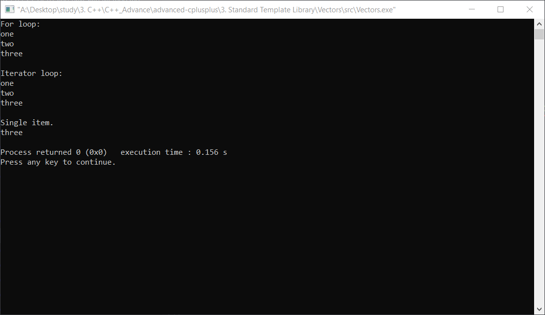
	cout << "For loop: " << endl;
	for(int i=0; i<strings.size(); i++) {
		cout << strings[i] << endl;
	}
	cout << endl;
	// .end() <- after the element
	// vector.end() <- end interator를 반환
	// vector.begin() <- beginning iterator 반환
	//
	cout << "Iterator loop: " << endl;
	//The auto keyword specifies that the type of the variable that is begin declared will automatically be deduced
	//from its initializer and for functions if their return type is auto then that will be evaluated by return type expression at runtime.
	// auto 키워드를 사용하면 초깃값의 형식에 맞춰 선언하는 인스턴스(뱐수)의 형식이 자동으로 결정된다.
	for(auto it = strings.begin(); it != strings.end(); ++it) {
		cout << *it << endl;
	}
	cout << endl;

	cout << "Single item." << endl;
	vector<string>::iterator it = strings.begin();
	//strings.begin()<- this will actually give us a thing called an iterator(반복자)
	//which points to the first element in the vector.
	//vector<string>::iterator it <- it is that equal to return value of string stop again

	it += 2;
	// so we gonna call the first vector + 2 index value

	cout << *it << endl;

	return 0;
}

Result

Vector and Memory

  • capacity is the size of the internal array that the vector is using and that size is going to increase as you add elements
  • we’ve reserve we precisely rated 20 elements. so capacity is 20
  • capacity 배열의 크기만 신경쓴다. 값은 신경안씀!
  • expenantionaly increase number of elements
  • proportional to the number of elements in the array if insert an element into a vector and it has to internally create a new array a bigger capacity and then copy the elements from the order rates.
  • how big our arrays going to get based on its current size and it crease the capacity based on that
  • capacity is completely different the size of capacity is the size of the internal rate it reserved the size the actual number of elements that are added to that vector
  • numbers.resize(100) <- only resize size of valuable.
  • reserve method, we want to reserve(적립하다.) memory and in turn on a rate increase size of capacity array.
  • numbers.clear() <- remove all of the element in the vector
  • doent change the capacity of the internal array
  • Capacity가 꽉차서 원소를 추가하게 되면 배열의 수는 더블로 늘어난다
  • Ex 사이즈 2에 원소가 하나 늘어나면 Capacity 가 4 가 되고 똑같이 원소가 또 추가 되면 8되고 ``` #include #include using namespace std;

int main() {

vector<double> numbers(0);
//specifiy the argument (0)

cout << "Size: " << numbers.size() << endl;

int capacity = numbers.capacity();
//.capacity is the size of the internal array that the vector is using and that size is
//going to increase as you add elements
cout << "Capacity: " << capacity << endl;
//we've reserve we precisely rated 20 elements. so capacity is 20
//capacity 배열의 크기만 신경쓴다. 값은 신경안씀!

for(int i=0; i<10000; i++) {

	if(numbers.capacity() != capacity) {
		capacity = numbers.capacity();
		cout << "Capacity: " << capacity << endl;
	}

	numbers.push_back(i);
}
// expenantionaly incresae number of elemenst
// propotiaonal to the number of elements in the array
// if insert an element into a vector and it has to internally create a new array
// a bigger capacity and then copy the elements from the order rates.
// how big our arrays going to get based on its current size
// and it crease the capacity based on that
// capacity is completely different the size of capacity is the size of the internal
// rate it reserved the size the actual number of elements that are added to that vector
numbers.reserve(100000);
//numbers.resize(100) <- only resize size of valuable.
//reserve method, we want to reserve(적립하다.) memory and in turn on a rate
//increase size of capacity array.
cout << numbers[2] << endl;
cout << "Size: " << numbers.size() << endl;
cout << "Capacity: " << numbers.capacity() << endl;

//numbers.clear() <- remove all of the element in the vector
//doent change the capacity of the internal array


return 0; }

> Result

<a href="https://postimg.cc/kVvY541T"><img src="https://i.postimg.cc/Dzt9B4q3/421321312.png" width="700px" title="source: imgur.com" /></a>

# Two Dimensional vectors
- Vector<> <- column
- Vector<vector<>> <- raw
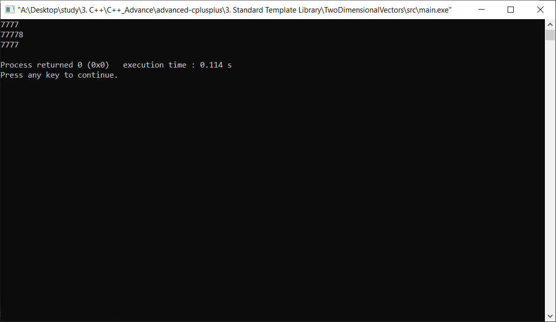
- grid( 3<- 3 raw , vector<int>(4,7) <- some value put)
- 3 space of raw, 4 space of column all value is 7


#include #include

using namespace std;

int main() { vector< vector > grid(3, vector(4, 7)); //Vector<> <- column //Vector<vector<>> <- raw //grid( 3<- 3 raw , vector(4,7) <- some value put) // 3 space of raw, 4 space of column

grid[1].push_back(8);

for(int row=0; row < grid.size(); row++) {
		for(int col=0; col < grid[row].size(); col++) {
			cout << grid[row][col] << flush;
			//grid[row] is the vector
			//and [col] is to access the elements in that particular row using
			//this column
		}

		cout << endl;
}

return 0; } ``` > Result

Sorting Vectors Deque Friend

  • Deque : 리스트의 양쪽 끝에서 삽입과 삭제를 모두 허용하는 자료의 구조. 이것은 스택과 큐의 자료 구조를 복합한 형태이다.

Deque

  • 덱은 벡터와 비슷하게 O(1) 으로 임의의 위치의 원소에 접근할 수 있으며 맨 뒤에 원소를 추가/제거 하는 작업도 O(1) 으로 수행할 수 있습니다.
  • 뿐만아니라 벡터와는 다르게 맨 앞에 원소를 추가/제거 하는 작업 까지도 O(1)O(1) 으로 수행 가능합니다.
  • 임의의 위치에 있는 원소를 제거/추가 하는 작업은 벡터와 마찬가지로 O(n)O(n) 으로 수행 가능합니다
  • 그렇다면 덱이 벡터에 비해 모든 면에서 비교 우위에 있는 걸까요?
  • 안타깝게도 벡터와는 다르게 덱의 경우 원소들이 실제로 메모리 상에서 연속적으로 존재하지는 않습니다.
  • 이 때문에 원소들이 어디에 저장되어 있는지에 대한 정보를 보관하기 위해 추가적인 메모리가 더 필요로 합니다.
  • 실제 예로, 64 비트 libc++ 라이브러리의 경우 1 개의 원소를 보관하는 덱은 그 원소 크기에 비해 8 배나 더 많은 메모리를 필요로 합니다).
  • 즉 덱은 실행 속도를 위해 메모리를 (많이) 희생하는 컨테이너라 보면 됩니다.
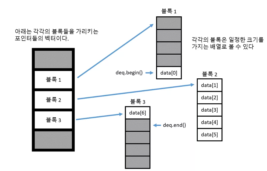
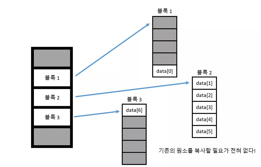
  • 벡터와는 다르게 원소들이 메모리에 연속되어 존재하는 것이 아니라 일정 크기로 잘려서 각각의 블록 속에 존재합니다.
  • 따라서 이 블록들이 메모리 상에 어느 곳에 위치하여 있는지 저장하기 위해서 각각의 블록들의 주소를 저장하는 벡터가 필요로 합니다.
  • 존의 벡터와는 조금 다르게, 새로 할당 시에 앞쪽 및 뒤쪽 모두에 공간을 남겨놓게 됩니다. (벡터의 경우 뒤쪽에만 공간이 남았지요) 따라서 이를 통해 맨 앞과 맨 뒤에 O(1) 의 속도로 insert 및 erase 를 수행할 수 있는 것입니다.
  • 그렇다면 왜 덱이 벡터 보다 원소를 삽입하는 작업이 더 빠른 것일까요?
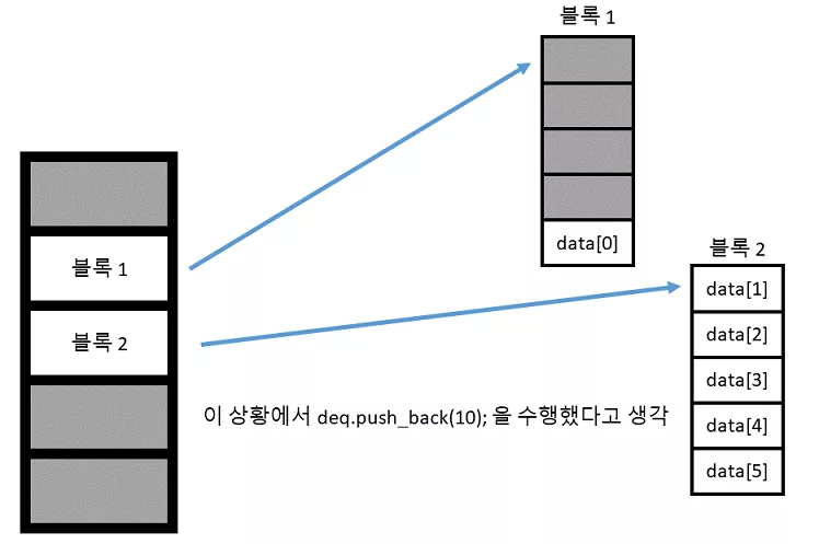
  • 위와 같은 상황에서 deq.push_back(10) 을 수행하였다고 생각해봅시다.
  • 그렇다면 단순히 새로운 블록을 만들어서 뒤에 추가되는 원소를 넣어주면 됩니다
  • 즉 기존의 원소들을 복사할 필요가 전혀 없다는 의미 입니다.
  • 반면에 벡터의 경우
  • 만약에 기존에 할당한 메모리가 꽉 차면 모든 원소들을 새로운 공간에 복사해야 합니다. 따라서 평균적으로 덱이 벡터보다 더 빠르게 작동합니다.
  • 물론 덱의 경우 블록 주소를 보관하는 벡터가 꽉 차게 되면 새로운 공간에 모두 복사해야 합니다.
  • 하지만 블록 주소의 개수는 전체 원소 개수 보다 적고 대체로 벡터에 저장되는객체들의 크기가 주소값의 크기보다 크기 때문에 복사 속도가 훨씬 빠릅니다.)
#include <iostream>
#include <string>
#include <vector>
#include <algorithm>

using namespace std;

class Test
{
	string name;
	int id;

public:
	Test(int id, string name) :
		id(id), name(name)
	{

	}

	bool operator<(const Test &other)  const {
		return name == other.name ? id < other.id : name < other.name;

		//?: <- is the conditional operator
		// condition ? result_if_true : result_if_false
		/* int qempty()
		{
            if(f==r)
            {
                return 1;
            }
            else
            {
                return 0;
            }
		}*/ // example of conditional operator
	}
	// because of for function??

	void print()
	{
		cout << id << ": " << name << endl;
	}

	friend bool comp(const Test &first, const Test &second);
	// friend function은 protect data/function 에 접근이 가능하다.
};

bool comp(const Test &first, const Test &second)
{
	return first.name < second.name;
}
// 알파뱃 순서로 정령한다.

int main(int argc, char const *argv[])
{

	vector<Test> tests;

	tests.push_back(Test(5, "Mike"));
	tests.push_back(Test(10, "Sue"));
	tests.push_back(Test(7, "Raj"));
	tests.push_back(Test(3, "Vicky"));

	sort(tests.begin(), tests.end(), comp);
	//comp is the funtion pointer

	for(int i = 0; i < tests.size(); i++)
	{
		tests[i].print();
	}

	return 0;
}

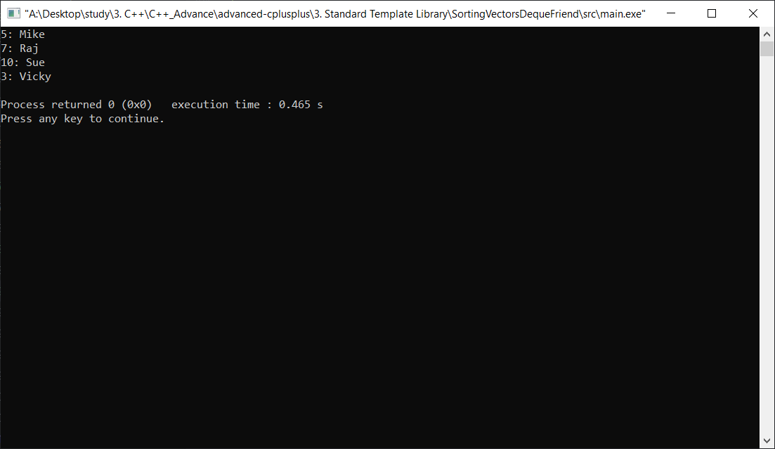
Result

REFERENCE

모두의코드

Comment  Read more

10. Value Function(2) & Bellman Equation

|

Value Function & The Bellman Equation

  • The full derivation(起源) can be tough if our probability skills are not yet strong enough

1. Expected Values

  • why is this strange to many people?
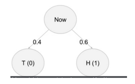
  • Consider a coin toss: Heads = Win, Tails = Lose
  • Numerically: H = 1, T = 0
  • suppose, P(W) = 60%
  • Expected Value is 0.6 x 1 + 0.4 * 0 = 0.6
  • The “Expected Value” is a “Value” I can “never expect”
  • What’s the point of expected values?
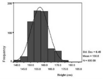
  • it tells us the mean/average (E.g. we gather up all the heights of students in the call and calculate the mean- no student may have the mean height, but it’s a useful statistic)
  • it doesn’t matter if a coin flip will never give me 0.6, it just an average
  • x is state()

2. probability Trees

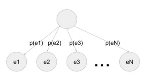
  • our expected reward is the weighted sum of each possible outcome(weighted by the probability at the corresponding branch)
  • the same concept extends to any number of possible outcomes
  • in general: Expected value = p(e1) x value(e1) + p(e2) x value(e2) + ….

3. Why are averages important?

  • A subsection(分部) of a tree is also a tree – recursion(递归)
  • After Arriving in this state, what happens next can be considered Random
  • Hence, we cannot say: “if i reach this state, i will get X reward”
  • we can only say: “if i reach this state, i will get X reward on average

4. A fundamental concept of The Value Function

  • At each state s, i will get a reward R
  • overall return G, is the sum of rewards i get
  • we want to be able to answer:
    • “if i am in state, s what is the sum of reward i will get in the future, on average?”
    • we say: V(s) = E(GIs)
  • “I” means “givens” - anything to the left is random/ right is not random
  • note : this is called a “conditional expectation”
  • Value Function is equal to Expected function of Total Return by state
  • Every Game we play is just a series of states and rewards
  • Let’s pretend everything is deterministic for now, e.g. E(3) = 3
  • The value of a state is just the sum of all future rewards(if they are deterministic)
    • V($s_1$) = $r_2$ + $r_3$ + $r_4$ + … + $r_N$
    • V($s_2$) = $r_3$ + $r_4$ + … + $r_N$
    • Key: V($s_1$) = $r_2$ + V($s_2$)
  • Discounted Version
    • V($s_1$) = $r_2$ + ɣ$r_3$ + ɣ$r_4$ + … + $r_N$
    • V($s_2$) = ɣ$r_3$ + ɣ$r_4$ + … + ɣ$r_N$
    • Key: V($s_1$) = $r_2$ + ɣV($s_2$)
    • (still assuming everything is deterministic)
  • In more general terms
    • Let’s make s = current state, s’=next state
    • Let’s make r = reward(reall means R(s,s’)- the reward i get from going from s to s’)
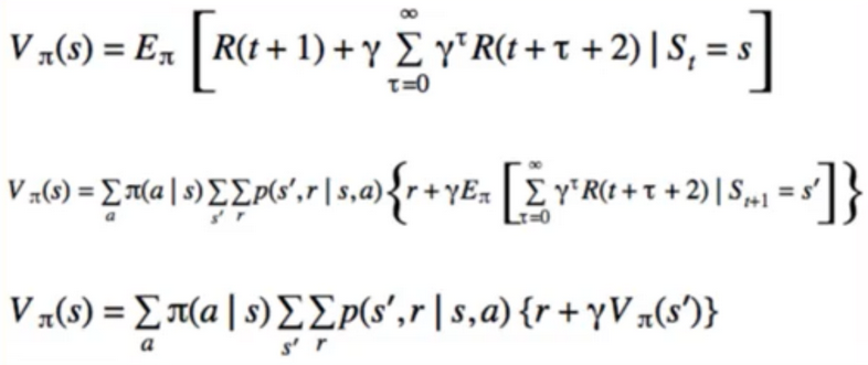
    • V(s) = E[r + ɣV(s’)]
    • this is the essence of the bellman equation
  • Expansion
    • V(s) = E[r + ɣE(r’+ɣV(s’’))]
    • V(s) = E[r + ɣE(r’+ɣE(r’‘+…))]
    • understanding this “Structure”
  • putting more details back in
    • s is “given” - we’ve already arrived here
    • V(s) = E[r + ɣV(s’) I s]
  • Expansion again
    • V(s) = state-value function
    • Q(s,a) = action-value function
    • Q(s,a) = E[GIs,a] = E[r + ɣV(s’) I s,a]
    • to understand how Q anv V are related, we need to look at policies(something that tells us what action a to do, given what state we are in)
  • we know earlier(informally) with tic-tac-Toe
  • if any discrepancies(差异) between then and now, consider everything from here onward to be more correct
  • Value Function is determined by a policy and has state “s” as parameter
  • only future rewards
  • value of all terminal states is thus 0
  • the state value of the terminal state in an episodic problem should always be zero, the value of a state is the expected sum of all future rewards when starting in that state and following a specific policy. for the terminal state, this is zero - there are no more rewards to be end 0
  • Recursiveness(递归性)

5. Some Algebra

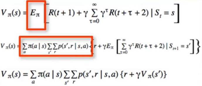
  • since the expected value is over π, that means we can express it as a possibility distribute
    • π = π(a I s)
  • the expected values are linear operators, so we can find each term one at a time
    • policy with in return action value in respect to state
    • reward and probabilty with return reward in respect to state and action
  • in terms of p(s’,r I s,a)
  • we can do this for anything
    • it’s just a general expression of expected values, we can use it on anything

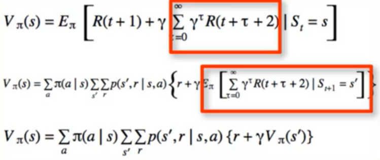
So let’s do it for all of V(s)

  • E(E(X)) = E(X)
  • we can do this infinity and it won’t change the answer
  • E(A+B) = E(A+E(B))
  • Therefore if i have one expected value like that, i can insert another expected value in there
  • Law of total expectation: E(X)=E(E(X I Y))
  • E(E(G(t+1) I ANY)) = E(G(t+1))
  • now we know that any condition or expectation could go in that spot
  • pick ANY = S(t+1) = s’
  • if i want to know what to do next i just look at what is the reward i get by going there whay is this has to do with how to find an optimal policy.
  • Key: No need to enumerate all possible future(which could be infinity long), in order to choose every action

6. Bellman Equation

  • Richard bellman
  • Pioneered “dynamic programming”
  • Bottom-up approach
  • DP(dynamic programming) is also one of the solution we’ll study for MDPs
  • State-value Fucntion
  • Action-value function
  • Space Required is quadratic: ISI x IAI

7. Bellman Equation by Example

  • Simple models with just a handful of states, easy to solve by hand
  • Big Picture perspective: All we want to do is “solve for V(S)”
  • ‘Value Function’ represent how good is a state for an agent to be in

Example 1

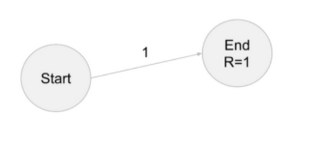
  • probability of going to end, from start, is 1
  • Reward for landing in end is 1
  • Discount factor ɣ = 0.9
  • Question: what problem are we solving again?
  • if we said, “find V(s)”, we are right
  • In particular, we want:
    • V(START)
    • V(End)
  • Try it ourselves before moving on
  • Remember “Value” is sum of all Future rewards
  • Value of Terminal state is always 0
  • V(end) = 0
  • V(start) = 1
  • Note: ɣ only applies to future rewards
  • V(start) = R + ɣ(End)

Example 2

  • Everything is still deterministic
  • Discount factor ɣ = 0.9
  • V(End)=0 (terminal state)
  • V(Mid)=1 (Takes the role of V(Start) From Example 1)
  • V(Start) = R(Start,Mid) + ɣV(Mid) = 0 + 0.9 x 1 = 0.9

Example 3

  • V(End) = 0 (unaffected)
  • V(Mid) = 1 (Also unaffected, only calculated from future rewards)
  • V(Star) = R(Start,Mid) + ɣV(Mid) = -0.1 + 0.9*1 = 0.8

Example 4

  • Start at S1
  • Discount factor ɣ = 0.9
  • Nuance: What do these Probabilities refer to?
  • we model games as MDPs - not just coin flips
  • as an intelligent agent, our policy tells me what action to do : π(a I s).
  • Important : Does not tell me where we go
  • p(s’,r I s,a) tells me where i end up
  • this example oversimplifies MDPs, but is easier to verbalize(用言语)
  • For these examples, we’ll consider the action to be “deciding where to go”
  • V(S4) = 0
  • V(S2) = 1
  • V(S3) = 1 (Same logic as previous examples)
  • V(S1) = p(S2 I S1)[R2+ɣV(S2)]+p(S3 I S1)[R3+ɣV(S3)] = 0.5(-0.2 + 0.91)+0.5(-0.3 + 0.91) = 0.65

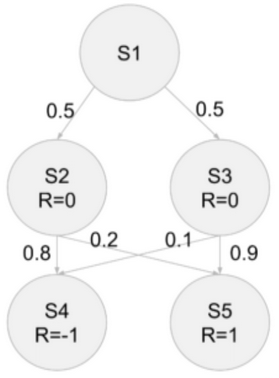
Example 5

  • V(S4), V(S5) =0 (Terminal)
  • V(S2) = p(S4 I S2)[R4 + ɣV(S4)] + p(S5 I S2)[R5 + ɣV(S5)] = 0.8-1 + 0.21 = -0.6
  • V(S3) = p(S4 I S3)[R4 + ɣV(S4)] + p(S5 I S3)[R5 + ɣV(S5)] = 0.1-1 + 0.91 = 0.8
  • V(S1) = p(S2 I S1)[R2 + ɣV(S2)] + p(S3 I S1)[R3 + ɣV(S3)] = 0.5(0.9-0.6) + 0.5(0.9*0.8)= 0.09

Example 6

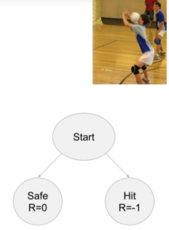
  • sperate policy randomness from state-arrival randomness
  • situation:
    • someone throws a ball at me
    • our action: either “duck” or “jump”
    • next possible states:
      • Get hit: R = -1
      • Don’t Get hit(safe): R = 0
  • the action cannot be “don’t get hit”
    • if one could simply choose not to get hit one would never lose
  • can aplly to any “real-life” scenario, e.g. starting a company
  • π(jump I start) = 0.5
  • π(duck I start) = 0.5
p(hit, reward = -1 I jump,start) = 0.8
p(hit, reward = 0 I jump,start) = 0
p(safe, reward = -1 I jump,start) = 0
p(safe, reward = 0 I jump,start) = 0.2
p(hit, reward = -1 I duck,start) = 0.2
p(hit, reward = 0 I duck,start) = 0.4
p(safe, reward = -1 I duck,start) = 0.6
p(safe, reward = 0 I duck,start) = 0.4
  • just marginalize over reward since they are really deterministic
p(hit, reward = -1 I jump,start) = 0.8
p(safe, reward = 0 I jump,start) = 0.2

p(hit, reward = 0 I duck,start) = 0.4
p(safe, reward = -1 I duck,start) = 0.6
  • as usual, V(safe) and V(hit) = 0

  • sanity(明智) check: we should have 4 things to sum over (2 x 2 - think of looping over all possibilities in code)
for brevity(简洁):
Don't show start condition
j = jump, d = duck

V(Start) = π(j)p(safe I j)*0 + π(j)p(hit I j) * (-1) + π(d)p(safe I j)*0 + π(d)p(safe I j)*(-1)

Example 7

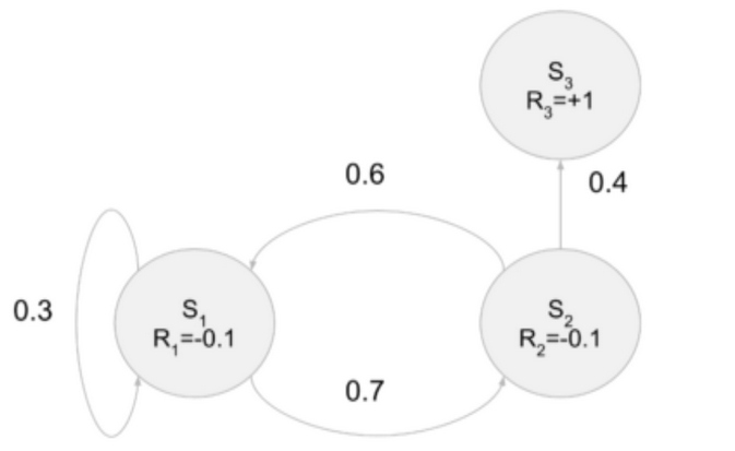
  • The Previous examples were easy: just work backwards
  • Now we have a cycle: no notion of “backwards”
  • Back to actions being “go to next state”
  • R1 = R2 = -0.1
  • Discount Factor ɣ = 0.9
V(s1) = p(s1 I s1)(R1+ɣV(s1)) + p(s2 I s1)(R2 + ɣV(s2))
V(s1) = 0.3(-0.1+0.9V(s1)) + 0.7(-0.1 + 0.9V(s2)) = -0.1 + 0.27V(s1) + 0.63V(s2)
V(s2) = p(s1 I s2)(R1+ɣV(s1)) + p(s3 I s2)(R3 + ɣV(s3))
V(s2) = 0.6(-0.1+0.9V(s1)) + 0.4(1 + 0.9V(s3)) = 0.34 + 0.54V(s1) + 0.36V(s3)
V(s3) = 0
V(s1) = -0.1 + 0.27V(s1) + 0.63V(s2)
V(s2) =0.34 + 0.54V(s1)
V(s3) = 0
  • this is linear system (3 equations, 3 unknowns)
0.1   = -0.73V(s1) + 0.63V(s2)
-0.34 = 0.54V(s1) - V(s2) + 0.36V(s3)
0     = V(s3)

  • of the form Ax=b x = np.linalg.solve(A,b)
  • V(s1) = 0.293
  • V(s2) = 0.498
  • V(s3) = 0

7. Bellman Equation Summary

  • “Working backwards method”
  • “Linear eqaution method”
  • big picture:
  • Get away from the idea that : “i need to try this on a finance data”, “i need to try this on a biology dataset”, etc.. algorithm doesn’t change, all it sees is a list of numbers
  • Rather, we want to know: “ What are scalable algorithms that solve this modelling problem?”

8. Optimal Policies & Optimal Value Functions

  • these are interdependent - a key concept in this course - lots of depth to this idea
  • we can talk about the relative “goodness” of policies

The Best Policy

  • optimal policy is the “best” policy
  • the policy for which there is no greater value function
  • Optimal Policies are not unique, optimal value functions are :

Relationship Between V and Q

  • Implementation advantage:
  • to find the best action, we must actually do it to find the best V(s’)
  • With Q, we simply need to Look up Q(s,a)

Bellman Optimality Equation

9. Implementing the Optimal Policy

  • Key point : Value Function already takes future rewards into account
  • Just greedily choose the action that yield the best next-state value V(s’)
  • requires look-ahead search
  • if we have Q(s,a), no need to look ahead, simply choose argmax
  • Q(s,a) thus effectively caches the look-ahead search results

10. step from Value Function to Optimal Policy and Q function

  • the value function depends on the policy by which the agent picks actions to perform. so if the agent uses a given policy π to select actions, the corresponding value function is given by :
  • among all possible value-functions, there exist an optimal value function that has higher value than other functions for all states
  • the optimal policy π is the policy that corresponds to optimal value function.
  • In addition to the state value-function, for Convenience RL algorithms introduce another function which is the state-action pair Q-Function. Q is a function of a state-action pair and returns a real value

11. MDP Summary

  • Purely Theoretical
  • MDPs
  • Policies
  • Returns-total future reward
  • Discounting future rewards with the discount rate, gamma
  • state-value function
  • action-value function
  • bellman equation
  • Bellman Optimality Equations
  • Next Section:
    • Finding V given a policy
    • Finding Optimal Policies and optimal values

Reference:

Artificial Intelligence Reinforcement Learning

Advance AI : Deep-Reinforcement Learning

Cutting-Edge Deep-Reinforcement Learning

Comment  Read more

28. Standard Template library(STL) - Map

|

Maps

  • 기본형태
    • map<key,value> : key와 value를 pair 형태로 선언합니다.
  • iterator(반복자)
    • begin() : beginning iterator를 반환
      • end() : end iterator를 반환
  • 추가 및 삭제
    • insert( make_pair(key,value) ) : 맵에 원소를 pair 형태로 추가
      • erase(key) : 맵에서 key(키값)에 해당하는 원소 삭제
      • clear() : 맵의 원소들 모두 삭제
  • 조회
    • find(key) : key(키값)에 해당하는 iterator를 반환
      • count(key) : key(키값)에 해당하는 원소들(value들)의 개수를 반환
  • 기타
    • empty() : 맵이 비어있으면 true 아니면 false를 반환
      • size() : 맵 원소들의 수를 반환
#include <iostream>
#include <map>
#include <string>

using namespace std;

int main() {

	map<string, int> ages;

	ages["Mike"] = 40;
	ages["Raj"] = 20;
	ages["Vicky"] = 30;

	ages["Mike"] = 70;
	//
	ages.insert(make_pair("Peter", 100));
	//pair<string, int> addToMap("peter",100);
	//ages.insert(addToMap);

	cout << ages["Raj"] << endl;
	// to find the techinical
	if(ages.find("Vicky") != ages.end()) {
		cout << "Found Vicky" << endl;
	}
	else {
		cout << "Key not found." << endl;
	}

	for(map<string, int>::iterator it = ages.begin(); it != ages.end(); it++) {
		pair<string, int> age = *it;

		cout << age.first << ": " << age.second << endl;
		// first and second the function in the map library
	}

	for(map<string, int>::iterator it = ages.begin(); it != ages.end(); it++) {
			cout << it->first << ": " << it->second << endl;
			// first and second is valuable the value of the ages by key and value.

		}


	return 0;
}

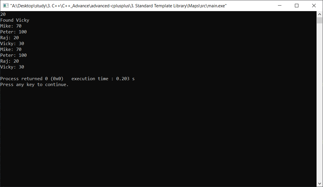
Result

Custom Objects as map Keys

Flush

  • 개발 된 Microsoft C/c + + 응용 프로그램에서는 cout 스트림 버퍼링 됩니다.
  • 즉, 버퍼를 플러시할 때까지 cout 스트림에 보낼 정보가 화면에 나타나지 않습니다.
  • 이 동작은 Visual C++ 4.2 및 이후 버전의 경우 이전 iostream 라이브러리를 사용할 때만 발생 합니다.
  • 네 가지 방법을 다음과 같이 cout 버퍼를 플러시할 수 있습니다.
    • Endl 조작자를 사용 하 여 줄 바꿈 문자를 출력 스트림에 삽입 버퍼를 플러시합니다. Endl 조작자를 사용 하 여 삽입 연산자를 다음과 같이 사용.
      • cout « … « endl;
      • Ostream 클래스 또는 플러시 조작자에 플러시 멤버 함수를 사용 합니다.
      • 플러시 조작자 버퍼를 플러시합니다 전에 스트림에 줄 바꿈 문자가 삽입 되지는 않습니다. 플러시 멤버 함수를 호출 하려면 다음과 유사한 코드를 사용.
        • cout.flush();
      • 플러시 조작자를 사용 하 여 삽입 연산자를 다음과 같이 사용.
        • cout « … « flush;

First and Second 함수

  • 구조체 템플릿 std::pair 는 두 가지 유형의 정확히 두 개의 반환 값을 함께 묶을 수 있습니다
#include <utility>
std::pair<int, int> foo(int a, int b) {
    return std::make_pair(a+b, a-b);
}
  • C ++ 11 이후 버전에서는 std::make_pair 대신에 초기화리스트를 사용할 수 있습니다 :
#include <utility>
std::pair<int, int> foo(int a, int b) {
    return {a+b, a-b};
}
  • 쌍의 first 및 second 구성원 개체를 사용하여 반환 된 std::pair 의 개별 값을 검색 할 수 있습니다.
std::pair<int, int> mrvs = foo(5, 12);
std::cout << mrvs.first + mrvs.second << std::endl;

Example

  • Map<person, int> people
  • Person first map and value is second map
  • Ex) [Person1, value1] [person2,value2]…
#include <iostream>
#include <map>
#include <string>

using namespace std;

class Person {
private:
	string name;
	int age;

public:

	Person() :
			name(""), age(0) {

	}

	Person(string name, int age) :
			name(name), age(age) {

	}
	// 상속
	//constructor need to initialize this
	//so thats why we use to initilaze the actual instance(기억장치 할당) variables in above
	//we dont have to provide any more implementation(실행)


	Person(const Person& other) {
		name = other.name;
		age = other.age;
	}

	//copy constoctur.

	void print() const {
		cout << name << ": " << age << flush;
	}

	//operator is just like +,-,<,>,!= 지정해주는
	// 리퍼런스 other에 대신 데이터를 받아 가동을 시켜준다.
	bool operator<(const Person &other) const {

		if (name == other.name) {
			return age < other.age;
		} else {
			return name < other.name;
		}
	}
};

int main() {
	map<Person, int> people;
	//map<key,value>

	people[Person("Mike", 40)] = 40;
	people[Person("Mike", 444)] = 123;
	people[Person("Sue", 30)] = 30;
	people[Person("Raj", 40)] = 20;

	for (map<Person, int>::iterator it = people.begin(); it != people.end();
			it++) {
		cout << it->second << ": " << flush;
		it->first.print();
		cout << endl;
	}
	// it need to bool operation becuase
	return 0;
}

Example 2

#include <iostream>
#include <map>
#include <string>

using namespace std;

class Person {
private:
	string name;
	int age;

public:

	Person() :
			name(""), age(0) {

	}
	// this is the default parameter of constructor.
	// this is the keep
	// member-wise <- in terms of(관해서) members(item associated with class instances)
	Person(string name, int age) :
			name(name), age(age) {

	}
	// this is necassary for 기억할당 in map function

	Person(const Person &other){
		cout << "Copy constructor running!" << endl;
		name = other.name; // 얕은복사
		age = other.age;  //깊은 복사
	}
	// copy constructor is a member function which initialize an obeject using another object of the same class
	// 복사생성자의 값을 복사 구성체에다가 받는다
	// 인트매인에서 객체에 주어진 값이 같지만 주소가 바뀌거나 생성자 호출을 하지 않기 떄문에 이와 같이
	// 새로운 공간 할당.


	void print() {
		cout << name << ": " << age << endl;
	}
};

int main() {
	map<int, Person> people;

	people[50] = Person("Mike", 40);
	people[32] = Person("Vicky", 30);
	people[1] = Person("Raj", 20);

	people.insert(make_pair(55, Person("Bob", 45 )));
	people.insert(make_pair(55, Person("Sue", 24 )));
	// copy constructor is called heres

	for (map<int, Person>::iterator it = people.begin(); it != people.end();
			it++) {
		cout << it->first << ": " << flush;
		it->second.print();
	}
// flush is sending a content and cleaning up the buffer
	return 0;
}

REFERENCE

모두의코드

Comment  Read more

9. Markov Decision Processes

|

Markov Decision Processes

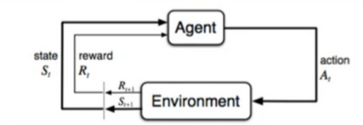
  • this section: formalize some RL concepts we already know about
  • Agent, Environment, action, state, reward, episode
  • Formal Framework: Markov Decision Processes(MDPs)

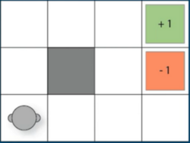
1. Typical Game by solving MDPs is GridWord

  • possible actions:
  • up,down,left,right
  • (1,1) -> wall,can’t go here
  • (0,3) -> Terminal(+1 Reward)
  • (1,3) -> Terminal(-1 Reward)
  • 12 Positions(w x h = 3 x 4 = 12)
  • 11 states (where the robot is)
  • 4 actions

2. Markov Property

  • Given a sequence:
  • Generally, this can’t be simplified:
  • First-order Markov:
  • second-order Markov:
  • Simple Example ``` Consider the sentence : “Let’s do a simple example” Given:”let’s do a simple” Predict the new word? Easy

Given: “simple” Predict the next word? not as easy

Given: “a” predict the next word? very difficult

is the Markov Property limiting? Not necessarily ```

3. Markov Property in RL

  • {S(t), A(t)} produces 2 things -> {S(t+1),R(t+1)}
  • Markov Property:
  • Convenience notation
  • joint on s’ and r, conditioned on 2 other variables
  • different from “usual” Markov: 1 RV(Random Variable) Conditioned on 1 other RV

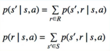
4. Other Conditional distributions

  • can be found using rules of probability
  • For pretty much all cases we’ll consider these will be deterministic
  • i.e. states will always give us the same reward
  • Action will always bring us to same next state
  • But, these distributions are part of the core theory of RL

5. Is the Markov Assumption limiting?

  • Not necessarily
  • Recent application: DeepMind used concatenation(一系列相关联的事物) of 4 most recent frames to represent state when playing Atari Games
  • State can be made up of anything from anytime past to current
  • Typically think of state right now = something we measure right now
  • Also, don’t need to use raw data(state can be features transformed from raw data)
  • Any input from agent’s sensors can be used to form state

6. Markov Decision Processes(MDPs)

  • Any RL task with a set of States, actions, and rewards, that follows the Markov Property, is a MDP
  • MDP is defined as the collection of
    • set of states
    • set of actions
    • set of rewards
    • State-Transition probability, Reward probability(as defined jointly(连带地) earlier)
    • Discount factor
  • Often written as a 5 tuples

7. Policy

  • One more piece to complete the puzzle - the policy(denoted by π)
  • Technically π is not part of the MDP itself, but it, along with the value function, form the solution
  • Left out until now because it’s a weird symbol
  • there’s no “equation” for it
  • how do we write epsilon-greedy as an equation? it’s more like an algorithm
  • the only exception is the Optimal policy, which can be defined in terms of the value function
  • think of π as shorthand for the algorithm the agent is using to navigate the environment

    8. State-Transition probability - p(s’|s,a)

  • State Diagram
  • p(s’ I s,a)
  • why is this stochastic? if i press “jump” button, doesn’t it always do the same thing?
  • Recall: state is only derived from what agent senses, it’s not the environment itself
  • State can be imperfect representation of environment
  • Ex) state could represent multiple configuration of environment
  • Ex) Blackjack - if we’re the agent, the dealer’s next card is not part of our state(but it is part of the environment)

9. Actions vs Environment

  • Typically we think of action like joystick inputs(up/down/left/right/jump) or Blackjack Moves(hit/stand)
  • Actions can be very board: how to distribute government funding
  • we are navigating an environment, we are the agent - what constitutes(구성하다) “us”?
  • Are our body? No
  • our body is part of the environment, our body doesn’t make decisions/learn
  • brain/mind does the learning

10. Total Reward & Future Reward

  • We are Interested in measuring total future reward
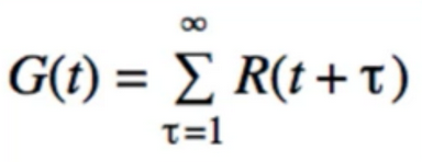
  • Everything from t+1 onward(继续的)
  • We call this the Return, G(t)
  • Note: does not count current reward R(t)

Future Reward

  • Imagine a very long task(thousands of steps)
  • is there a difference between getting a reward now, and getting the same reward 10 years from now?
  • think finance
  • $1000 today is worth less than $ 1000 10 years ago
  • Would you rather get $1000 today or $1000 10 years from now? choose today

11. Discount Factor

  • Gamma = 1: don’t care how far is the future reward is, weight all equally
  • Gamma = 0: truly greedy, only try to maximize immediate reward
  • Usually we choose something close to 1, i.e 0.9
  • Short episode task: maybe don’t discount at all
  • “the further we look into the future, the harder it is to predict”

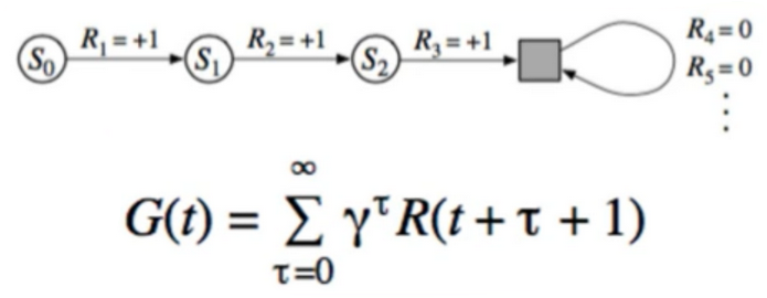
12. Merging Continuous and episode tasks

  • why count up to infinity? Aren’t we doing episodic tasks?
  • yes, but math is easier with infinity. so can make them technically equivalent(相等的)

번외

  • (Epsilon Greedy는 주사위 한번 던져서 결정하고 그 action 다음번에 사용하는 것이 on Policy)
  • (Q-Learning은 다음 Step에서 실제로 사용할 action과 상관 없이 Max Q 취하기 때문에 off policy)
    • 각 지점에서 계속 최적값을 찾으면서 Future Reward 计算
    • 벨멘 방정식을 이용하여 반복적으로 Q함수를 근사시킬 수 있음
  • (Sarsa, 다음번에 게임에 넣어줄 action을 미리 계산해서 사용)
  • Reinforcement Learning Two Problem
    • Credit Assignment Problem
    • Exploration-exploitation
  • DQN Property
    • Target Q function
      • 학습 대상이 되는 Q함수가 학습이 되면서 계속 바뀌는 문제
      • Learning Q-Fucntion from Gradient Descent
      • 일정 스텝 될 때마다 Q 함수의 가중치를 타켓 Q함수에 업데이트
    • Replay Memory
      • 학습의 재료가 되는 Sample 저장소
      • 즉시 훈련하지 않고, 메로리 저장
      • 일정 수의 Samplr을 랜덤으로 꺼내 학습
    • Q-function made by ANN
      • DQN은 인공신경망으로 Policy function을 Approximate
    • Q function of DQN 특징
      1. Model Free :
        • 모델이 없고 샘플로 부터 직접적으로 정책을 근사화
        • 대부분 ANN을 활용한 훈련으로 Dimension Curse에 벗어난다.
      2. Off-Policy
        • Learn thing from another agent’s action
        • 타겟 정책과 행동 정책 나눈다.
        • Target policy : 우리가 강화학습 에이전트에게 가르치기 위한 기준이 되는 정책
        • 행동 Policy : 탐험을 하며 새로운 행동을 만들어 내는 정책 - 두가지 폴리시를 다루어야 함으로 구현하기 어려움
      3. MiniBatch
        • 많은 데이터 중 임의로 샘플을 뽑아 학습시키는 것
        • 연속적인 샘플들 간의 강한 상관관계를 제거
      4. Value-Based Reinforcement Learning
        • at first, Let Value Function Approximating to make a Policy
      5. Decaying Epsilon-Greedy
        • at first, Random Act -> random act to be reduced gradually -> when it became 1% of random action, it stop
        • Two Hyper parameter: (1) Exploration_fraction : 언제까지 감소 시킬 것인가? Default 0.5(Timesteps의 50%가 될 때까지 랜덤 액션 취할 확률 이 줄어든다) (2) Exploration_final_eps : 최종 입실론 값, 기본값 0.01(0.01이 되면 감소가 줄어들고, 값을 유지한다.)

        Reference:

        Artificial Intelligence Reinforcement Learning
        Advance AI : Deep-Reinforcement Learning

        Cutting-Edge Deep-Reinforcement Learning

Comment  Read more