Introduction

• Now that we know the basic data structures, we can begin using them to build different, more helpful data structures.

Why is it Important?

• Stacks are used for a variety of operations in computer science. They can do anything from helping to navigate through a maze, to helping traverse a graph.

Lesson Notes

• Stacks are a data structure that are built off the backs of other data structures. They work off a set of important rules.

• These rules are usually applied to either a linked list or array. It’s like a specialization. Through the rules we are able to create a specialized structure with new pros and cons.

• A stack works like a stack of trays in the cafeteria. You always grab from the top, not the bottom. This means you will have a relationship where the most recent element that has come, will be the first serviced.

• Let’s say 100 items come into a stack in order. So 1 is inserted, then 2, then 3, etc. In this case, 100 would be “served” first, then 99, then 98, then 97 and so on. This is helpful for something like an undo system on an application. Every step you make is inserted onto the stack. Then whenever you want to undo, you just “pop” off the top of the stack to go back in time.

• With this pattern, we now have what is known as a “Last in First Out (LIFO)” relationship. This is also commonly referred to as a “Last Come, First Served(LCFS)” relationship.

• Going along with the terminology. These are some key terms to know when working with stacks and queues.

• Pop - To remove an element from a stack. (Can sometimes be used for queues).

• Push - To insert an element onto a stack. (Can sometimes be used for queues).

• Enqueue - To insert an element onto a queue

• Dequeue - To remove an element from a Queue.

• FIFO - Means “First in First Out” It’s the technical term for a queue-like data structure.

• LIFO - Means “Last In First Out”. It’s the technical term for a stack-like data structure.

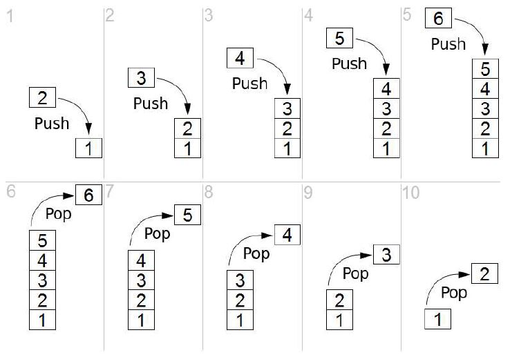
• Let’s take a look at how a stack operates through an example:

• Notice how it looks like we are “stacking” books or trays up. We keep stacking. Then when we want to remove one, we take it off the top. We never remove from anywhere else in a stack!

• Now, if we kept popping and pushing in a loop, we would get a situation where number 1 could potentially never be touched again. For this reason, these aren’t typically used for scheduling purposes. Imagine if you used a stack to run your computer. Old windows would be frozen indefinitely as new requests keep getting serviced first.

• In the next set of lessons, we will cover a data structure that is more apt to deal with situations like this.

Introduction

• We can improve linked lists by making them doubly-linked as well as creating a tail pointer.

Why is it Important?

• Giving us the ability to go forward AND backwards can be very helpful in a linked list. Also having the ability to start from the back can not only speed up access time, but it can make insertions to the back constant time.

Lesson Notes

Doubly-Linked List

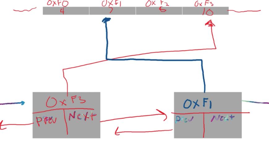
• A doubly-linked list is the same as a singly-linked list with one major difference, instead of just a “next” pointer within each node, there is also a “previous” pointer. Note, this will typically increase the memory needed for the list, as each node now has another pointer to keep track of.

• This however allows one to not only go forwards in the list, but also to go backwards in the list. This can be helpful for a large amount of applications.

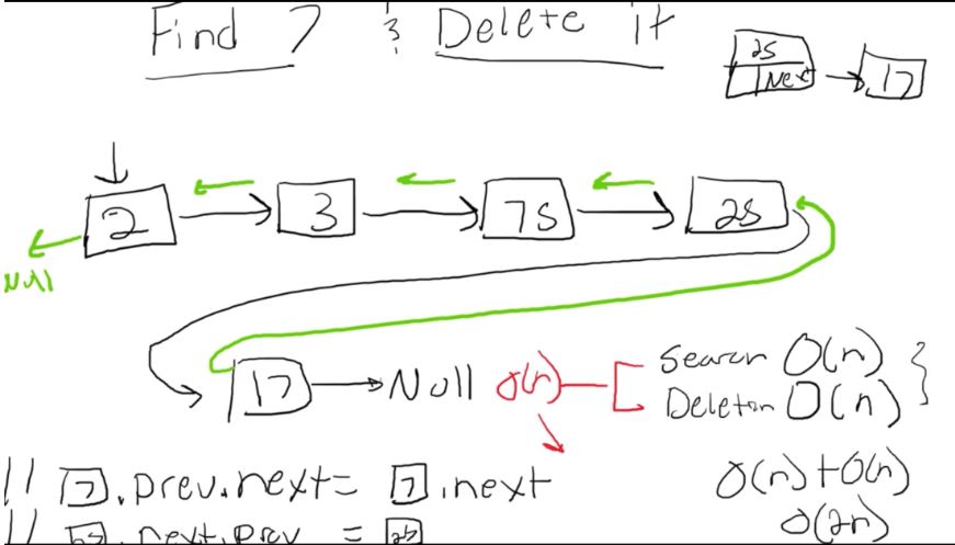
• For example, let’s say we want to print out the list back to front. With a singly-linked list, we would need to go to the last element, and print it. We would then have to start back at the beginning, go to n-1, then to n-2, and so on. We would have to keep restarting from the beginning.

• So if we had the H->E->A->P example. If we wanted to print PEAH, we would have to first access H->E->A to get to P. We would then have to access H->E to get to the A and so on. This would make it so we would have to touch 10 pieces of data just to print out 5 pieces. This would scale up as well. If the array was 5 large, it would require 15 touches, 6 would require 21, and 7 would require 28.

• The formula for this is actually known as a linear summation, or n(n+1) / 2, where n is the size of the list. So with our H->E->A->P example, it would be n=4, or 4(4+1) / 2 => 4(5)/2 => 20/2 => 10.

• If we multiply the n through, we get (n^2 + n) / 2, which you guessed it, shows us it’s an n^2 formula.

• If the list was doubly-linked however, we could go to the end of the list, print and move backwards until we get back to the front.

• This means this particular operation will be reduced from O(n^2) to O(n), quite a change

Tail Pointer

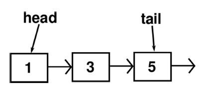
• A tail pointer is a small addition that can improve the deletion and insertion to the back of the list. By default, we have a “head” pointer. This, as seen in the picture above, points to the beginning of a list. It is used to give us a node to start our traversals from. Without it, we would have no way of getting to the beginning of the list, and therefore the list would be lost in memory.

• We however can also create another pointer, a “tail” pointer. This will point directly to the very last node added to the list.

• How does this help us? Well think of the two cases in which we want to delete or add information to the back of the list. Without a tail pointer we have to traverse the entire list until we get to the end, which by default is an O(n) operation

• So in the previous example H<->E<->A<->P (<-> signifies doubly-linked). Even with it being doubly-linked, it would still take O(n) operation to get to the back, and then O(n) operation to print from back to front. This would create O(2n) as the final run time. (This is simplified down to O(n) sure, but efficiency does matter at some point

• With a tail pointer however, we can just start directly on the end, and then add or delete from there. This takes the O(n) operation and brings it back to O(1). So now our print back to front will require a O(1) + O(n) operation, which is just a natural O(n) timing.

• Insert (Back): O(n) -> O(1)

• Delete (Back): O(n) -> O(1)

• So with two small additions, we have taken an operation that would have been O(n^2), and reduced it down to an actual O(n) timing. This is what computer science is all about. Coming up with solutions to help make programs more efficient.

Introduction

• Linked Lists are a core data structure that can link data together from multiple locations

Why is it Important?

• Linked Lists help us link data together from separate locations. In this way they are infinitely scalable and can contain multiple different types of data. This gives us a flexibility that arrays don’t give us.

Lesson Notes

Nodes

• Nodes are the building blocks of Singly Linked Lists. They are a data structure which holds a few key pieces of information.

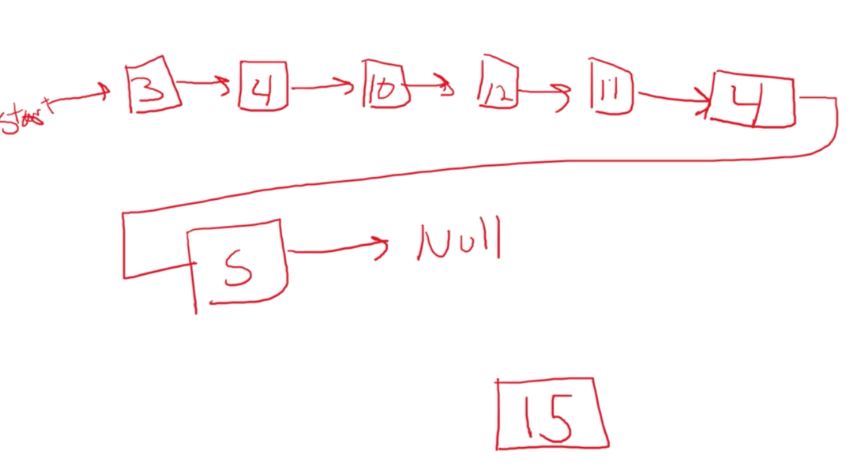
• The node usually contains a piece of data (a number, letter, location, etc) and then pointers t other nodes. In a singly-linked list it contains a pointer to the next node in the array. If it is at the end of the array, then it just points to NULL, which means nothing.

Linked List

• The very first node is designated as the “head” of the linked list. It is the node that is always pointed to when we call our linked list. This head is important, without it, we would lose our entire linked list.

• An important difference between linked lists and arrays is that the data in the linked list aren’t directly accessible.

• For example, if we had an array of tempArray = [H,E,A,P], we could access the P by calling tempArray[3]. This would instantly return us the P.

• With a linked list however, we can’t do that. We only have the first node, and then where that node points to. This means that we have to traverse the entire list before we get to the P. So, if we want the P element, we will have to touch the H, E, and A before we get to it.

• This means Linked Lists search times are typically slower than that of an array, even if the list is sorted, as there is no way to jump to a certain point.

Linked List Run Times

• Insert(Rand): O(n) - To insert at a particular location, one has to traverse the list up to that point to insert there.

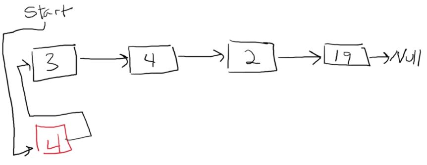
• Insert(Front): O(1) – We just move the head pointer to the new node and point the new node at the old head.

• Insert(Back): O(n) – We will have to traverse the entire array to get to the back. (We will find a way to improve this a little bit later)

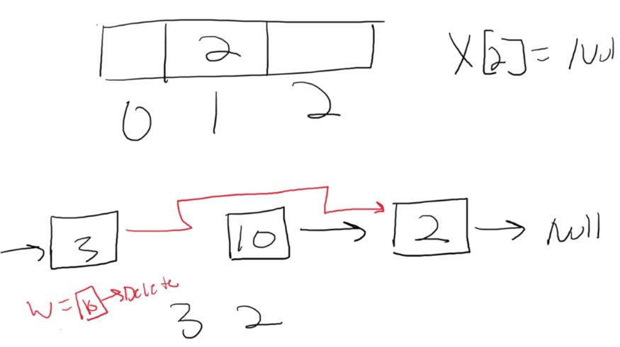
• Delete(Random): O(n) – We must traverse the length of the element we want to delete

• Delete(Front): O(1) – Just as easy as inserting, just have to remove the first element and repoint the head pointer

• Search(Sorted): O(n) – Doesn’t matter if it’s sorted or not. We at worst have to traverse the entirety of the list to find the element. (And if the element isn’t in the list, we have to traverse the entire list to figure that out. )

• Search(Unsorted): O(n) – Exactly the same as the Sorted.

Introduction

• Arrays can be improved from basic fixed sized arrays. These improvements can help make the arrays more flexible and efficient.

Why is it Important?

• Through these improvements we are able to dynamically store data, as well as decrease the insertion time and deletion times.

Lesson Notes

Circular Array

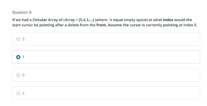
• One of the major problems with a typical array is that we could reach O(n) whenever we tried inserting or deleting into the front. The entire array had to be shifted, causing a lot of data to be touched that didn’t really need to be touched

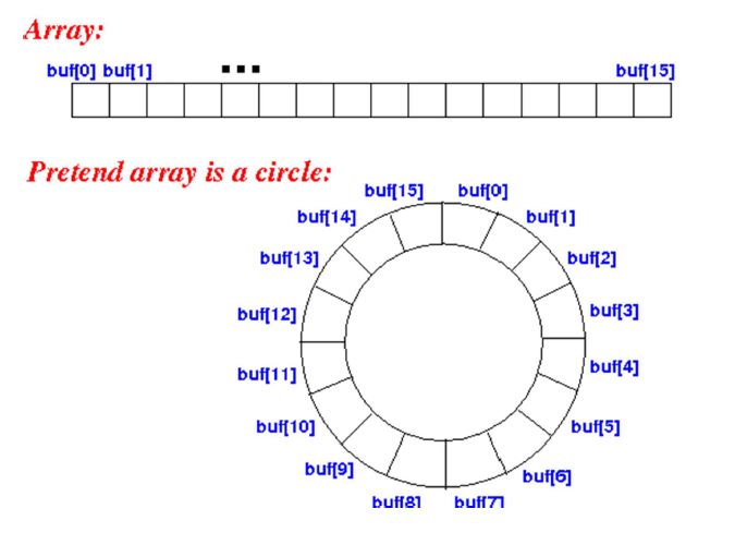
• To improve this, we pretend that the array is circular. This makes it so we never need to shift data.

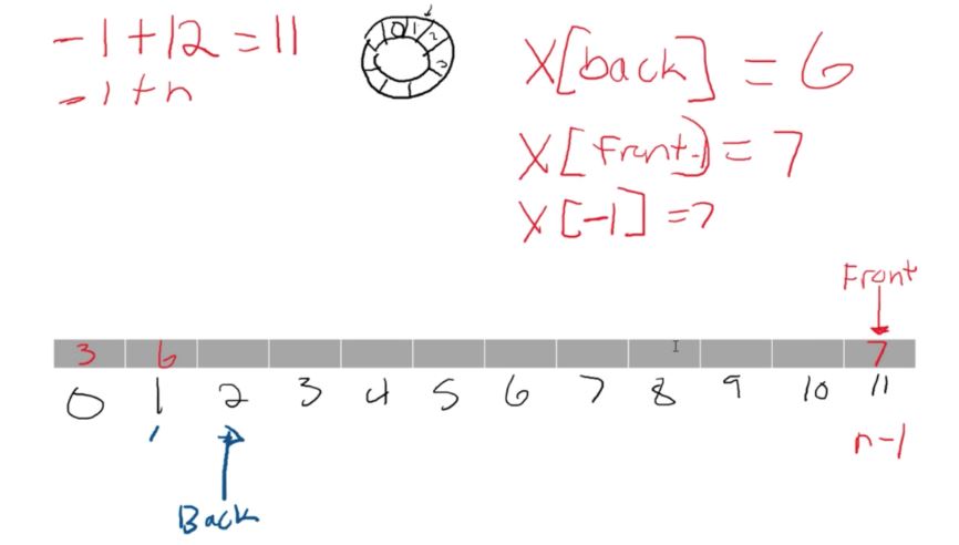
• So how do we pretend it’s circular? We create two cursors. A “start” cursor, which points to the beginning of the array, and an “end” cursor which points to the end of the array. These cursors are then adjusted when an element is deleted or added

• For example, let’s say we had some data in buff[0] that we wanted to delete. If we look at the typical horizontal array above, you will notice that when we delete this data, we will end up having to shift everything backwards to fill in the hole.

• However, with the circular array, what we do is to move the “front” cursor to buff[1]. This makes buff[1] our new beginning of the array. We can now add or delete anything, and instead of moving the data, we just move the cursor around.

• At some point the beginning of the array might be at buff[13] and the end might be at buff[6]. It just depends on how data is added and removed. Overall though, since we are only moving the location of the cursor, our run time improves to O(1) from O(n).

Dynamic Arrays

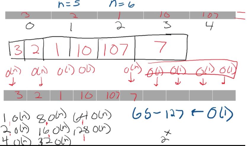
• A dynamic array gives us the ability to expand our array whenever we run out of room. This means we don’t need to know how much data is being input beforehand, making it a lot more “real-world” friendly.

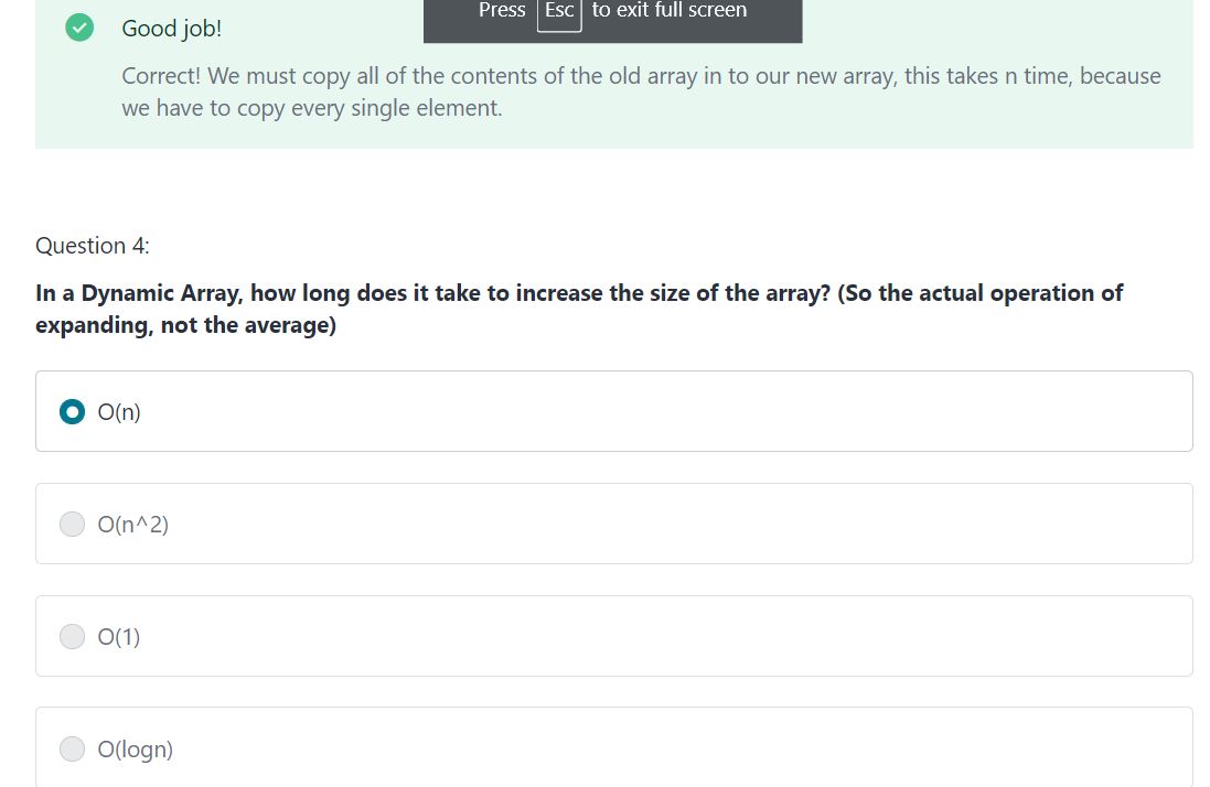
• Expanding our array each time we run out of data however runs in O(n) time. This is because once an array is allocated, it can’t be expanded. So what we do is create a new array with a new size, and then transfer over all of the contents from the previous array.

• This though requires we touch every single piece of data in the array, making the O(n) time. We can however improve this if we think about the problem a little bit further.

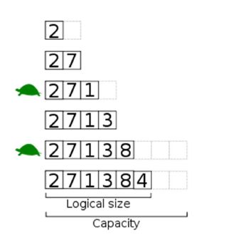
• Instead of increasing the size of the array by 1 each time when we run out of data, we can instead double the size of the array.

• For this, we use the terms logical size, and physical size. The logical size is how many pieces of data are actually allocated in the array. The physical size is the size of the array itself. So what we want to do, is every time our logical size reaches our physical size, we want to double the physical size.

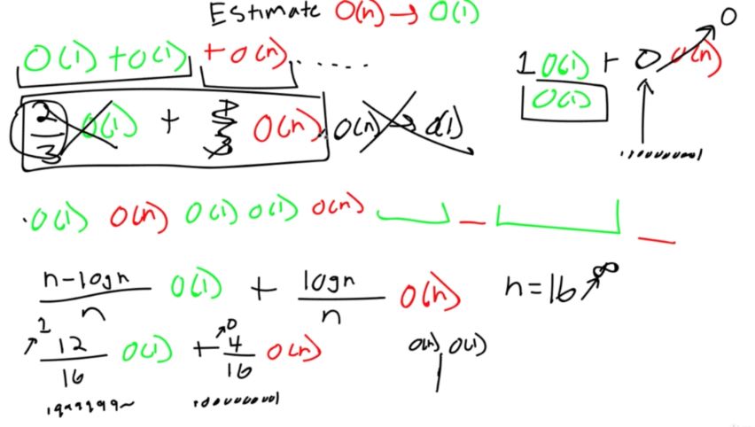
• This doubling provides a less and less frequent use of the O(n) copying operation, which overall leads to something called an amortized O(1) relationship. Amortize here just means averaged. This means is that it is technically O(n) because of the copy operation, but when averaged out to infinity, it more closely resembles that of O(1). Because of this, we can say it’s basically O(1).

• There is also a space-time complexity that needs to be thought of with this problem. The more you allocate after each “full” insert, the more chance there is of wasted space. It may speed up the run time, but may cost you a lot of storage space.

• For example, let’s say you have an array with 65,536 slots that gets filled up. If we want to add another element to this, we will then have an array which is 131,072 elements big. That is a gigantic leap. So this is usually optimized depending on the program

• This can all be expanded a bit farther. With some clever ingenuity(聪明才智), you can actually create a dynamic circular array, combining the best of everything mentioned.

• This array would just be a dynamic array with front and end cursors. This would allow you to delete and add in constant time, and also to make sure that when the array runs out of room it wouldn’t take up much time either.

Array address

Quiz

Introduction

• Arrays are a way of storing data in a linear sequence. This creates a fast-organized data structure

Why is it Important?

• Arrays are used everywhere. Because of their easy design and quick recall, they are widely used to store information during program execution. They can also be used to build more advanced data structures like stacks and queues.

Lesson Notes

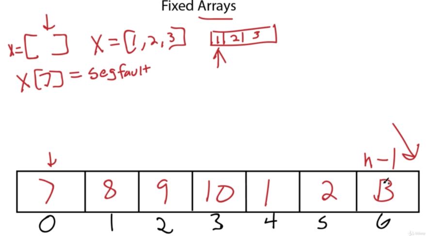
• Fixed arrays are the most basic version of an array. They are created with a fixed size and stick to this size throughout their execution

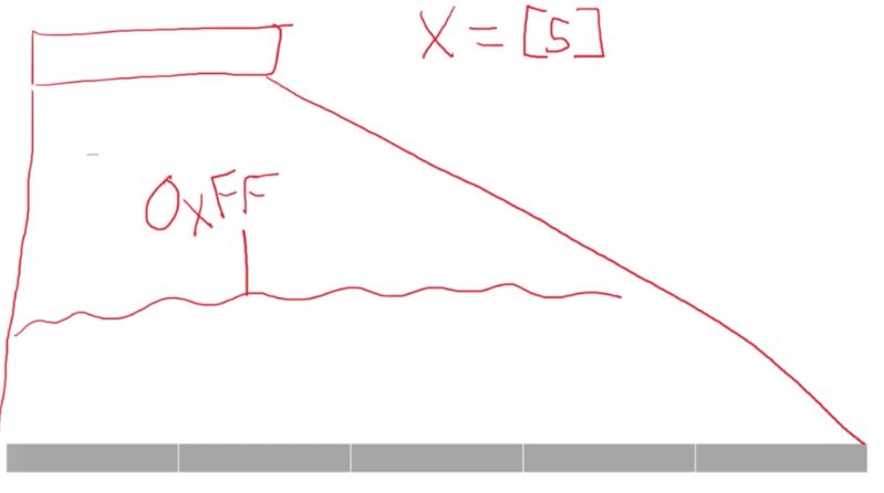
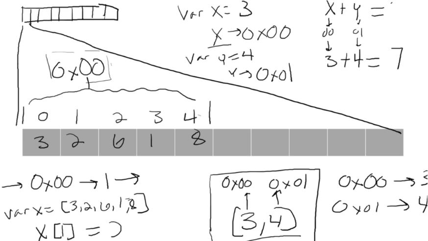
• Ox00 는 메모리 address 주소

• 정해진 어레이 크기에 넘어가는 수를 구하려고 하면, SegFault가 이러난다.

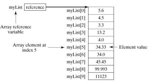
• An array works by allocating a section of memory for storage. Then whenever we call the array, it returns the location of start of the array. We can then apply the appropriate index number to get to any point in that array instantly.

• For example, in the figure above, the array myList is created and references the very beginning of the array. You can see this through the “reference” box that points to before the first element of the array.

• We can then put a number in the [] after myList to get a specific element of the array. So if we put myList[5] we would get in return 34.33.

Run Times

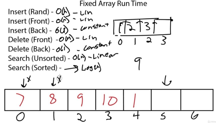
• Insertion Random: O(n) – It’s easy to insert randomly anywhere in the array. Getting to the location of insertion take O(1) time. However, if you want to preserve order, there is a chance you will have to move O(n) elements to put the number there. Therefore, it’s O(n).

• The reason we use n is because it will show us how our program might react differently to different amounts of data. We as computer scientists never know how many pieces of data our programs are going to handle. So instead, we look at how our program is going to grow with different amounts of inputs.

• Insertion Front: O(n) – Inserting in the front of an array will usually take O(n) time, as you have to shift up to n elements backwards to insert properly.

• Insertion Back: O(1) – Nothing has to be shifted, so you can accomplish this in O(1) time.

• Deletion Random: O(n) – Deleting randomly from the array is just like inserting randomly. You can get to and remove the element in O(1) time. However, if you need to delete an element and not create a hole, then this becomes O(n) as you will need to shift everything to cover the hole.

• Deletion Front: O(n) – Same as Insertion, a shift of up to n elements will be required.

• Search Unsorted: O(n) – If the array is unsorted, there is no way of knowing where the element is going to be. So at worst case, it’s going to be a search of the entire array to find the element.

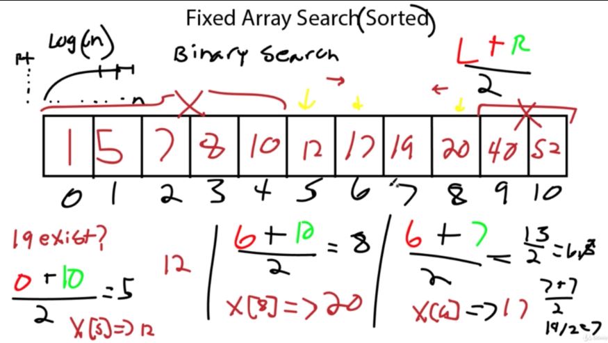
• Search Sorted: O(logn) – If the array is sorted, we can keep cutting the array in half to find the element we are searching for. This means it will take at most logn operations to find our element. (Reverse exponential).